5 Subscripting

Vectorized arithmetic and subscripting are two cornerstones of R programming. Review section 4.2 for several examples where subscripting has been used. In this chapter subscripting is studied in detail. Specifically, the following two related topics are studied:

Extracting parts of an object by using subscripting.
The combination and rearranging of data within data structures like matrices, dataframes and lists.

5.1 Subscripting with vectors

The different types of subscripting with vectors are summarized in Table 5.1:

Table 5.1: Different types of subscripting vectors.
Type	Effect	Example
empty	Extract all values	`x[ ]`
integer, positive	Extract all values specified by the subscript	`x[c(2:5,8,12) ]`
integer, negative	Extract all values except those specified by the subscript	`x[–c(2:5,8,12) ]`
logical	Extract those values for which subscript is TRUE	`x[x > 5 ]`
character	Extract those values whose names attributes correspond to those specified by the subscript	`x[c("a","d") ]`

Logical subscripting provides a very powerful operation in R. A logical subscript is a vector of TRUEs and FALSEs that must be of the same length as the object being subscripted e.g.

state.x77[ , "Area"] > 80000  
#>        Alabama         Alaska        Arizona       Arkansas 
#>          FALSE           TRUE           TRUE          FALSE 
#>     California       Colorado    Connecticut       Delaware 
#>           TRUE           TRUE          FALSE          FALSE 
#>        Florida        Georgia         Hawaii          Idaho 
#>          FALSE          FALSE          FALSE           TRUE 
#>       Illinois        Indiana           Iowa         Kansas 
#>          FALSE          FALSE          FALSE           TRUE 
#>       Kentucky      Louisiana          Maine       Maryland 
#>          FALSE          FALSE          FALSE          FALSE 
#>  Massachusetts       Michigan      Minnesota    Mississippi 
#>          FALSE          FALSE          FALSE          FALSE 
#>       Missouri        Montana       Nebraska         Nevada 
#>          FALSE           TRUE          FALSE           TRUE 
#>  New Hampshire     New Jersey     New Mexico       New York 
#>          FALSE          FALSE           TRUE          FALSE 
#> North Carolina   North Dakota           Ohio       Oklahoma 
#>          FALSE          FALSE          FALSE          FALSE 
#>         Oregon   Pennsylvania   Rhode Island South Carolina 
#>           TRUE          FALSE          FALSE          FALSE 
#>   South Dakota      Tennessee          Texas           Utah 
#>          FALSE          FALSE           TRUE           TRUE 
#>        Vermont       Virginia     Washington  West Virginia 
#>          FALSE          FALSE          FALSE          FALSE 
#>      Wisconsin        Wyoming 
#>          FALSE           TRUE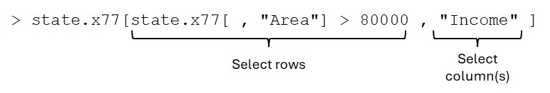

x <- c(10, 15, 12, NA, 18, 20)
is.na (x)
#> [1] FALSE FALSE FALSE  TRUE FALSE FALSE
x[is.na (x)]
#> [1] NA
x[!is.na (x)]
#> [1] 10 15 12 18 20
mean (x)
#> [1] NA
mean (x[!is.na (x)])
#> [1] 15
mean (na.omit (x))
#> [1] 15

Logical subscripting allows finding the indices of those elements in a vector that meet a certain condition e.g.

(1:length (rownames (state.x77)))[state.x77[ ,"Income"] > 5000]
#> [1]  2  5  7 13 20 28 30 34

and to find the corresponding names of the states

rownames(state.x77)[
  (1:length (rownames(state.x77)))[state.x77[ ,"Income"] > 5000]]
#> [1] "Alaska"       "California"   "Connecticut" 
#> [4] "Illinois"     "Maryland"     "Nevada"      
#> [7] "New Jersey"   "North Dakota"

In addition to extracting elements, the above subscripting operations can also be used to modify selected elements of a vector e.g. changing NA-values to zero:

x
#> [1] 10 15 12 NA 18 20
x[is.na (x)] <- 0
x
#> [1] 10 15 12  0 18 20

When the right-hand side of the assignment above is a scalar value, each of the selected values will be changed to the specified scalar value; if the right-hand side is a vector, the selecting values will be changed in order, recycling the values if more values were selected on the left-hand side than were available on the right-hand side.

5.2 Subscripting with matrices

Element and submatrix extraction of matrices are discussed below.

Revise the use of matrix(), names(), dim() and dimnames().
A matrix in R is an array with two indices. Arrays of order two and higher can be constructed with the function dim() or array().

Let, for example, $\mathbf{a}$ be a vector consisting of $150$ elements. The instruction

dim(a) <- c(3, 5, 10)

or the instruction

a <- array (a, dim = c(3, 5, 10))

constructs a $3 \times 5 \times 10$ array.

Matrices can therefore be formed as above, but the function matrix() is usually easier to use.
The elements of a $p$-dimensional array can also be extracted using the one-index or two-index method as described below.

The subscripting methods described in section 5.1 can also be applied to both the first or second dimension of a matrix where the first dimension refers to the rows and the second dimension to the columns of the matrix.
Note that the elements of a matrix can be referred to by the two-index method above or by a one index method. When the one index method is used it is assumed that the matrix has first been strung out column-wise into a vector.

testmat.a <- matrix (c (17, 40, 20, 34, 21, 12, 14, 57, 
                        78, 37, 29, 64), nrow = 4)
testmat.a
#>      [,1] [,2] [,3]
#> [1,]   17   21   78
#> [2,]   40   12   37
#> [3,]   20   14   29
#> [4,]   34   57   64
testmat.b <- matrix (c (17, 40, 20, 34, 21, 12, 14, 57, 
                        78, 37, 29, 64), nrow = 4, byrow = TRUE)
testmat.b
#>      [,1] [,2] [,3]
#> [1,]   17   40   20
#> [2,]   34   21   12
#> [3,]   14   57   78
#> [4,]   37   29   64

Comment on the difference between testmat.a and testmat.b.

testmat.a[2,3]   # Two index matrix reference
#> [1] 37
testmat.a[10]   # One index matrix reference
#> [1] 37

Write a function to convert a one-index to a two-index matrix reference. Give an example of the usage of your function.
Write a function to convert a two-index to a one-index matrix reference. Give an example of the usage of your function.

Consider the following example to form submatrices:

testmat <- matrix(1:50, nrow = 10, byrow = TRUE)
testmat[1:2, c (3, 5)]
#>      [,1] [,2]
#> [1,]    3    5
#> [2,]    8   10
testmat[1:2, 3]
#> [1] 3 8
testmat[1:2, 3, drop=FALSE]
#>      [,1]
#> [1,]    3
#> [2,]    8

Notice the difference between testmat [1:2, 3] and testmat [1:2, 3, drop = FALSE]. The first command results in the output to be given in the form of a vector while the optional drop = FALSE in the second command retains the matrix structure of the output. This distinction can have serious consequences when a procedure expects a matrix argument and not a vector.
Notice also that the output of both testmat[1:2,3] and testmat[3, 1:2] has a similar form: R makes no distinction between column vectors and row vectors; all one-dimensional collections of numbers are treated identically.
Apart from using vectors as subscripts to a matrix, a matrix can also be used as a subscript to a matrix. There are two cases:
1. a numeric subscripting matrix and
2. a logical subscripting matrix.

Case A

Here the subscripting numeric matrix must have exactly two columns: the first provide row indices and the second column indices.

If used on the right-hand side of an expression the result of a case A subscripting is a vector containing the values specified by the subscripting matrix.
If used on the left-hand side of an assignment a numeric matrix first selects those elements specified by its row and column indices; then these values are replaced one by one with the objects specified by the right-hand side of the assignment.

Here is an example of case A subscripting with the subscript matrix on the right-hand side of the assignment:

xmat <- matrix (1:25, nrow = 5)
xmat
#>      [,1] [,2] [,3] [,4] [,5]
#> [1,]    1    6   11   16   21
#> [2,]    2    7   12   17   22
#> [3,]    3    8   13   18   23
#> [4,]    4    9   14   19   24
#> [5,]    5   10   15   20   25
superdiag.index <- matrix (c (1:4, 2:5), ncol = 2, byrow = FALSE)
superdiag.values <- xmat[superdiag.index]
superdiag.values
#> [1]  6 12 18 24

Case A subscripting with the numeric subscript matrix on the left-hand side of the assignment:

subscript.mat <- matrix (c(1:3, 1:3, rep(1,3), rep(2,3)), ncol=2)
subscript.mat
#>      [,1] [,2]
#> [1,]    1    1
#> [2,]    2    1
#> [3,]    3    1
#> [4,]    1    2
#> [5,]    2    2
#> [6,]    3    2
xx <- matrix(NA, nrow=3,ncol=2)
xx 
#>      [,1] [,2]
#> [1,]   NA   NA
#> [2,]   NA   NA
#> [3,]   NA   NA
xx[subscript.mat] <- c(10,12,14,100,120,140)
xx
#>      [,1] [,2]
#> [1,]   10  100
#> [2,]   12  120
#> [3,]   14  140

Case B

The logical subscripting matrix must be in size exactly similar to that matrix it is subscripting and will select those values corresponding to a TRUE in the subscripting matrix.

Case B with logical subscripting matrix at right-hand side of assignment:

testmat
#>       [,1] [,2] [,3] [,4] [,5]
#>  [1,]    1    2    3    4    5
#>  [2,]    6    7    8    9   10
#>  [3,]   11   12   13   14   15
#>  [4,]   16   17   18   19   20
#>  [5,]   21   22   23   24   25
#>  [6,]   26   27   28   29   30
#>  [7,]   31   32   33   34   35
#>  [8,]   36   37   38   39   40
#>  [9,]   41   42   43   44   45
#> [10,]   46   47   48   49   50
aa <- testmat[testmat < 12]
aa
#>  [1]  1  6 11  2  7  3  8  4  9  5 10

Note that the selected elements are placed column-wise in a vector.

Case B with logical subscripting matrix at left-hand side of assignment:

testmat[testmat < 12] <- 12
testmat
#>       [,1] [,2] [,3] [,4] [,5]
#>  [1,]   12   12   12   12   12
#>  [2,]   12   12   12   12   12
#>  [3,]   12   12   13   14   15
#>  [4,]   16   17   18   19   20
#>  [5,]   21   22   23   24   25
#>  [6,]   26   27   28   29   30
#>  [7,]   31   32   33   34   35
#>  [8,]   36   37   38   39   40
#>  [9,]   41   42   43   44   45
#> [10,]   46   47   48   49   50

In order to restrict assignment to a subset of a matrix two sets of subscripts are needed. See example below:

testmat <- matrix(1:50, nrow=10, byrow=TRUE)
testmat[, c(1,3)][testmat[,c(1,3)] <12] <- 12
testmat
#>       [,1] [,2] [,3] [,4] [,5]
#>  [1,]   12    2   12    4    5
#>  [2,]   12    7   12    9   10
#>  [3,]   12   12   13   14   15
#>  [4,]   16   17   18   19   20
#>  [5,]   21   22   23   24   25
#>  [6,]   26   27   28   29   30
#>  [7,]   31   32   33   34   35
#>  [8,]   36   37   38   39   40
#>  [9,]   41   42   43   44   45
#> [10,]   46   47   48   49   50

Study the use of functions row() and col() in constructing logical matrices.

5.3 Extracting elements of lists

Note the use of list() to collect objects into a list while elements are extracted with $

the function names(),
the single square brackets [ ] and
the double square brackets [[ ]].

Study the following example carefully:

my.list <- list(el1 = 1:5, 
                el2 = c("a", "b", "c"), 
                el3 = matrix(1:16, ncol = 4), 
                el4 = c(12, 17, 23, 9))
my.list
#> $el1
#> [1] 1 2 3 4 5
#> 
#> $el2
#> [1] "a" "b" "c"
#> 
#> $el3
#>      [,1] [,2] [,3] [,4]
#> [1,]    1    5    9   13
#> [2,]    2    6   10   14
#> [3,]    3    7   11   15
#> [4,]    4    8   12   16
#> 
#> $el4
#> [1] 12 17 23  9
my.list$el2
#> [1] "a" "b" "c"
mode (my.list$el2)
#> [1] "character"
my.list[el2]
#> Error: object 'el2' not found
my.list["el2"]
#> $el2
#> [1] "a" "b" "c"
mode (my.list["el2"])
#> [1] "list"
my.list[["el2"]]
#> [1] "a" "b" "c"
mode (my.list[["el2"]])
#> [1] "character"

Note: The above example shows that using the single pair of square brackets for subscripting a list always result in a list object to be returned. This is often the cause of an error message. See the example below.

my.list[1]
#> $el1
#> [1] 1 2 3 4 5
mode (my.list[1])
#> [1] "list"
my.list[[1]]
#> [1] 1 2 3 4 5
mode (my.list[[1]])
#> [1] "numeric"
my.list[3][2,4]
#> Error in my.list[3][2, 4]: incorrect number of dimensions
my.list[[3]][2,4]
#> [1] 14
my.list$el3[2,4]
#> [1] 14
mean (my.list[4])
#> Warning in mean.default(my.list[4]): argument is not
#> numeric or logical: returning NA
#> [1] NA
mean (my.list[[4]])
#> [1] 15.25
mean (my.list$el4)
#> [1] 15.25

Explain the differences and similarities between the symbols [ ], [[ ]] and $ when subscripting lists.

5.4 Extracting elements from dataframes

Note the use of data.frame() for creating dataframes. A dataframe has a rectangular structure similar to a matrix but differs from a matrix in that its columns are not restricted to contain the same type of data. Each of its columns must contain the same sort of data but some columns can be numerical while others are factors for example.
Explain the difference between the objects created by the following two instructions:

my.matrix <- matrix (c (17, 40, 20, 34, 21, 12, 14, 57,
                        78, 37, 29, 64), nrow = 4, ncol = 3)
my.dataframe <- data.frame ( c(17, 40, 20, 34, 21, 12, 14, 57,
                               78, 37, 29, 64), nrow = 4, ncol = 3)

Note the following

class(my.matrix)
#> [1] "matrix" "array"
class(my.dataframe)
#> [1] "data.frame"
is.list(data.frame)
#> [1] FALSE
mode(my.matrix)
#> [1] "numeric"
mode(data.frame)
#> [1] "function"

A sample of the behaviour of dataframes

my.dataframe.2 <- data.frame (C1 = c('a', 'b', 'c', 'd'), 
                              C2 = c(5, 9, 23, 17), 
                              C3 = c(TRUE, TRUE, FALSE, TRUE))
my.dataframe.2
#>   C1 C2    C3
#> 1  a  5  TRUE
#> 2  b  9  TRUE
#> 3  c 23 FALSE
#> 4  d 17  TRUE
my.dataframe.2[ ,1:2]
#>   C1 C2
#> 1  a  5
#> 2  b  9
#> 3  c 23
#> 4  d 17

Dataframe behaves like a matrix

my.dataframe.2$C1
#> [1] "a" "b" "c" "d"

Dataframe behaves like a list

as.matrix(my.dataframe.2)
#>      C1  C2   C3     
#> [1,] "a" " 5" "TRUE" 
#> [2,] "b" " 9" "TRUE" 
#> [3,] "c" "23" "FALSE"
#> [4,] "d" "17" "TRUE"

Explain what has happened above.

The above examples show that a dataframe can be considered as a cross between a matrix and a list. Therefore, subscripting of dataframes generally can be performed using the basic techniques available for matrices and lists.
An alternative technique is to extract the elements of a list by using the functions attach() and names(). This technique is especially of importance in statistical modelling. What is a potential danger of this technique when attaching dataframes? This danger can be avoided by using with(). Is this also true when modelling is performed?
Review section 2.3. Study the help file of the function with(). What important usage has with()?

5.5 Combining vectors, matrices, lists and dataframes

What is the result of the command

my.list <- vector ("list", k)?

Recall the function c() for creating vectors. When c() is used to combine a numeric vector and a character vector the result is a vector of mode “character”. Similarly, using c() to combine a vector with a list results in a list.
If list() is used to combine two or more vectors or lists the result is a list of all the objects.
The function unlist() can be used to convert all the elements of a list into a single vector.

my.list
#> $el1
#> [1] 1 2 3 4 5
#> 
#> $el2
#> [1] "a" "b" "c"
#> 
#> $el3
#>      [,1] [,2] [,3] [,4]
#> [1,]    1    5    9   13
#> [2,]    2    6   10   14
#> [3,]    3    7   11   15
#> [4,]    4    8   12   16
#> 
#> $el4
#> [1] 12 17 23  9
unlist(my.list)
#>  el11  el12  el13  el14  el15  el21  el22  el23  el31  el32 
#>   "1"   "2"   "3"   "4"   "5"   "a"   "b"   "c"   "1"   "2" 
#>  el33  el34  el35  el36  el37  el38  el39 el310 el311 el312 
#>   "3"   "4"   "5"   "6"   "7"   "8"   "9"  "10"  "11"  "12" 
#> el313 el314 el315 el316  el41  el42  el43  el44 
#>  "13"  "14"  "15"  "16"  "12"  "17"  "23"   "9"

Explain the above output.

Review the functions cbind(), rbind(), append(), data.frame(), dim(), dimnames(), names(), colnames(), rownames(), nrow() and ncol().

5.6 Rearranging the elements in a matrix

Study the usage of the functions matrix(), t() and diag(). These functions are useful to form submatrices of a matrix or to rearrange matrix elements. Note again the argument byrow = of matrix().

5.7 Exercise

Write an R function to check if a given matrix is symmetric.
Write an R function to extract (i) the row(s) and (ii) the columns containing the maximum value in the matrix. Note that provision must be made that the maximum value can occur in more than one row (column). Furthermore, both the indices and actual values of the rows (columns) must be returned. Illustrate the usage of your function with a suitable example.
Describe the variables in the built-in data set LifeCycleSavings. Is this data set in the form of a matrix or a dataframe?
Use subscripting to find the largest proportion of over 75 in those countries with a dpi of less than 1000 in the LifeCycleSavings data set. Also determine the country(ies) having this pop75 value.
Consider the LifeCycleSavings data set.
1. Use subscripting to find the mean aggregate savings for countries with a percentage of the population younger than 15 at least 10 times the percentage of the population over 75.
2. Also find the mean aggregate savings for countries where the above ratio is less than 10.
3. Use function t.test() to test if mean aggregate savings are different for the above two groups.
4. Use notched box plots for an approximate test.

First, carefully study the output obtained in (iii) and (iv). Then interpret/discuss this output in detail.

Consider the state.x77 data set and the variable state.region. Find the state with the minimum income in each of the regions defined in state.region.

4 Introducing traditional R graphics

6 Revision tasks