8 Vectorized programming and mapping functions

In this chapter we continue the study the art of R programming. An important topic is a set of tools operating on objects like matrices, dataframes and lists as wholes.

8.1 Mapping functions to a matrix

What is understood by a mapping function and of what use are such functions?
The function apply().
1. What three arguments are required?
2. Suppose the third argument is a function. How are the arguments of this function used within apply()?

What is the result of the instruction apply(is.na(x),2,all)?
What is the result of the instruction x[ ,!apply(is.na(x), 2,all)]?
What is the result of the instruction x[ ,!apply(is.na(x), 2,any)]?

Set the random seed to 137921. Obtain a matrix \(\mathbf{A}:10 \times 6\) of random \(n(0, 1)\) values. Use apply() to find the \(10\%\) trimmed mean of each row.

The function sweep().
1. What arguments are required?
2. What are the similarities and differences between the arguments of sweep() and apply()?
3. Normalise the columns of a given matrix to have zero means and unit variances using scale(), apply() and sweep(). Which method is the fastest?
The function ifelse().

The usage is illustrated in the following diagram.

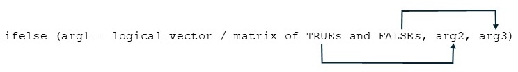
Note the difference between the function ifelse() and the control statement: if - else.
What arguments are required?
Study the help file in detail.

The function outer().
1. What arguments are required?
2. Revise our previous example of outer() when constructing a perspective plot with persp().
Work through the following examples and note in particular how the above functions are used together:
1. Find the maximum value(s) in each column of the LifeCycleSavings data set.
2. Use apply() together with cut() to divide each column of the LifeCycleSaving data set into low, medium and high.
3. Use apply() to plot each column of the LifeCycleSaving data set against the ratio of pop75 to pop15 on the x-axis.
4. Use apply() to find the coefficient of variation of each column of the LifeCycleSaving data set.
5. Use apply() together with cbind() and rbind() to obtain a table of the minimum and the maximum values of each column of the LifeCycleSaving data set.
6. Repeat (v) using the airquality data set with and without the elimination of the NAs by using an appropriate function definition in the call to apply().
7. Use sweep() to convert the LifeCycleSaving data set into standardized scores. Could apply() also be used for this task? Discuss.
8. Use ifelse() to convert negative values in a given vector to zero leaving positive values and missing values unchanged. Illustrate.

8.2 Mapping functions to vectors, dataframes and lists

Study the functions lapply(), sapply() and split().
Carefully study what is produced by the command

lapply (split (data.frame (state.x77),   
               cut (data.frame (state.x77)$Illiteracy, 3)), pairs)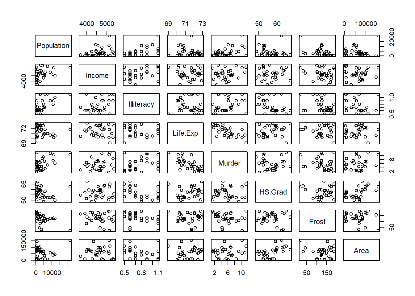

#> $`(0.498,1.27]`
#> NULL
#> 
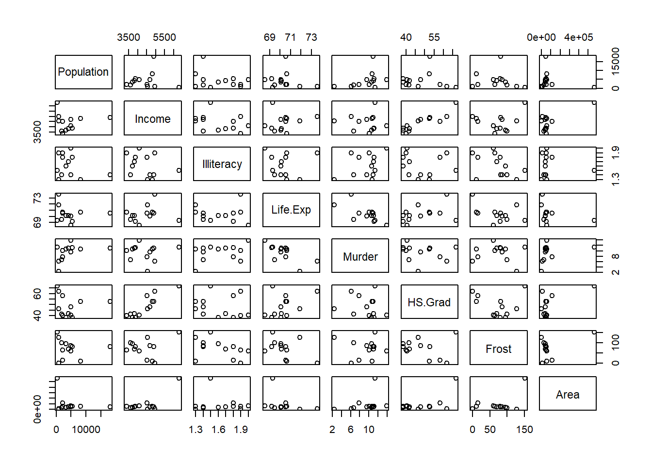
#> $`(1.27,2.03]`
#> NULL
#> 
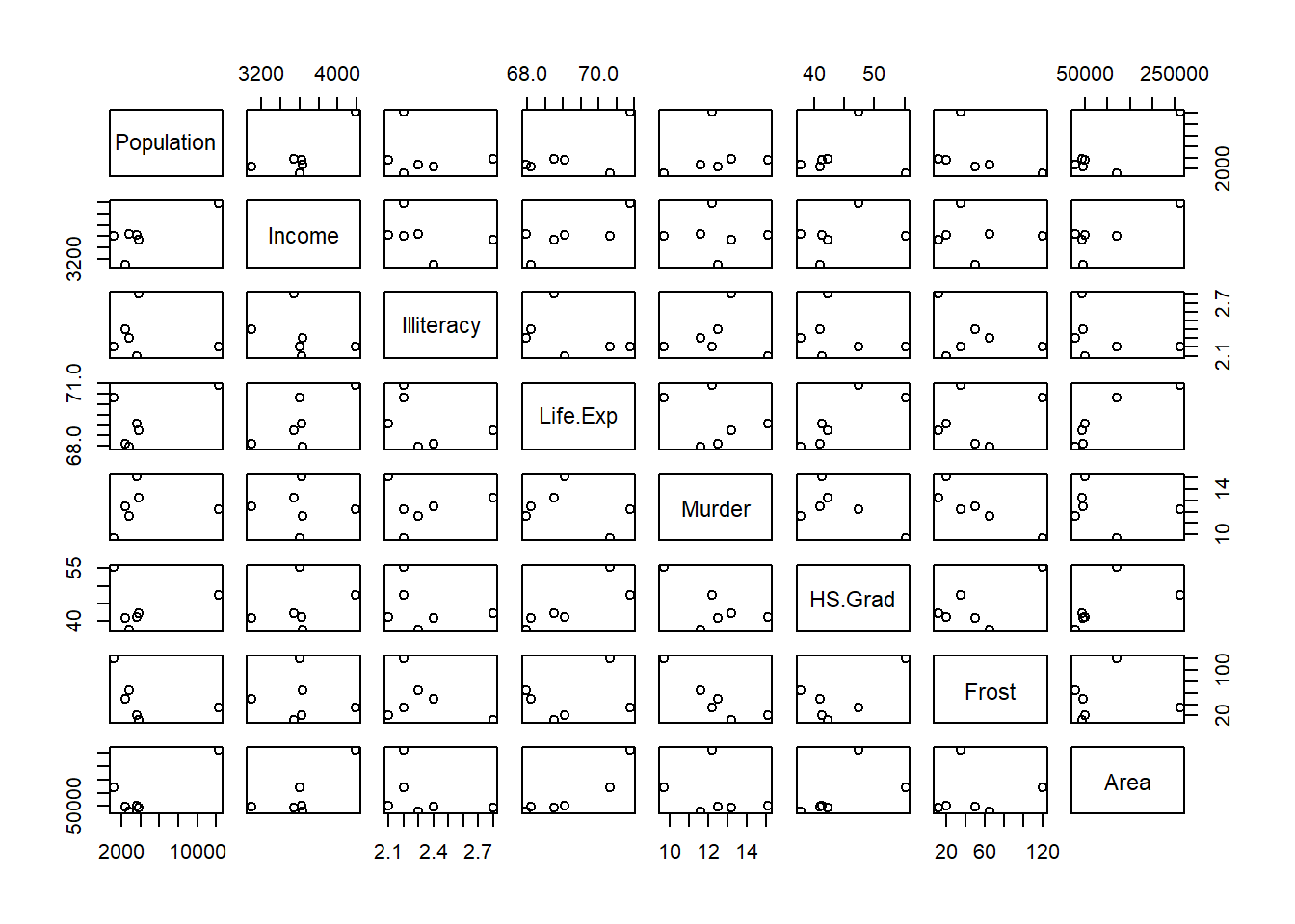
#> $`(2.03,2.8]`
#> NULL

Note: in order to see all graphs in the R-GUI it is necessary to issue the command

par(ask=TRUE)

before calling the function lapply().

Use lapply() to produce histograms of each of the variables in the state.x77 data set such that each histogram has as title the correct variable name. The \(x\)- and \(y\)-axis must also be labelled correctly.

8.3 The functions: `mapply()`, `rapply()` and `Vectorize()`

To apply a function to more than one list, mapply() is a multivariate version of sapply(). The first argument to mapply() is a function followed by the arguments for that function. The first argument function is applied to each of the elements in the following arguments.

mapply (function (x,y,z) {x+y+z}, x = c(2, 3), y = c(4,5), z = c(1,8))
#> [1]  7 16
mapply (function(x,y,z) { list (min (c(x,y,z)), max (c(x,y,z))) }, 
        x = c(2, 3), y = c(4, 5), z = c(1, 8))
#>      [,1] [,2]
#> [1,] 1    3   
#> [2,] 4    8

Study the help-files of rapply() and Vectorize().

8.4 The mapping function tapply() for grouped data

Study the arguments of tapply().

Consider the LifeCycleSavings data set. Create an object ddpigrp that groups the LifeCycleSavings data into four groups G1, G2, G3 and G4 such that G1 members have ddpi within \((0, 2.0]\), G2 members have ddpi within \((2.0, 3.5]\), G3 members have ddpi within \((3.5, 5.0]\), and G4 members have ddpi larger than \(5.0\). Use tapply() to obtain the mean aggregate personal savings of each of the groups defined by ddpigrp.
If it is needed to break down a vector by more than one categorical variable, a list containing the grouping variables is used as the second argument to tapply(). Illustrate this by finding the mean aggregate personal savings of the groups in ddpigrp broken down by the pop15 rating.

In order to use tapply() on more than one variable simultaneously apply() can be used to map tapply() to each of the variables in turn. Study the following command and its output carefully:

ddpigrp <- cut (LifeCycleSavings$ddpi, 
                breaks = c(0, 2, 3.5, 5, max(LifeCycleSavings$ddpi)),
                labels = paste0 ("G", 1:4))
apply (LifeCycleSavings [,c (1, 3, 4)], 2, function(x) 
                                           tapply (x, ddpigrp, mean)) 
#>           sr    pop75       dpi
#> G1  7.855385 1.790769  712.1677
#> G2  8.230625 2.456250 1497.0731
#> G3 11.959000 3.189000 1569.4910
#> G4 11.831818 1.834545  584.6964

If tapply() is called without a third argument it returns a vector of the same length than its first argument containing an index into the output that normally would be produced. Illustrate this behaviour and discuss its usage.

8.5 The control of execution flow statement if-else and the control functions `ifelse()` and `switch()`

The primary tool for conditional computations is the if statement. It takes the form:

if (logical condition evaluating to either TRUE or FALSE)
    {
     First set consisting of one or more R expressions
    }
else
    {
     Second set consisting of one or more R expressions
    } 
Expression3

In the above the else and its accompanying expression(s) are optional.
If-else statements can be nested.
Remember that the function ifelse() operates on objects as wholes as illustrated below:

xx <- matrix(1:25, ncol=5)
xx
#>      [,1] [,2] [,3] [,4] [,5]
#> [1,]    1    6   11   16   21
#> [2,]    2    7   12   17   22
#> [3,]    3    8   13   18   23
#> [4,]    4    9   14   19   24
#> [5,]    5   10   15   20   25
ifelse(xx < 10, 0, 1)
#>      [,1] [,2] [,3] [,4] [,5]
#> [1,]    0    0    1    1    1
#> [2,]    0    0    1    1    1
#> [3,]    0    0    1    1    1
#> [4,]    0    0    1    1    1
#> [5,]    0    1    1    1    1

Note that the function match() can be used as an alternative to multiple if-else statements in certain cases. The function match() takes as first argument a vector, x, of values to be matched and as second argument, table, a vector of possible values to be matched against. A third argument nomatch = NA specifies the return value if no match occurs. See the example below:

match (c (1:5, 3), c (2, 3))
#> [1] NA  1  2 NA NA  2
match (c (1:5, 3), c (2, 3), nomatch = 0)
#> [1] 0 1 2 0 0 2
match (c (1:5, 3), c (3, 2), nomatch = 0)
#> [1] 0 2 1 0 0 1

The following example provides an illustration of the usage of match():

month.num <- 5:9
month.name <- c("May", "June", "July", "Aug", "Sept")
new.vec <-  month.name [match (airquality [, "Month"], month.num)]
out <- data.frame (airquality [ ,1:5], MonthName = new.vec, 
                   Day = airquality$Day)
out[c(1:5,148:153), ]
#>     Ozone Solar.R Wind Temp Month MonthName Day
#> 1      41     190  7.4   67     5       May   1
#> 2      36     118  8.0   72     5       May   2
#> 3      12     149 12.6   74     5       May   3
#> 4      18     313 11.5   62     5       May   4
#> 5      NA      NA 14.3   56     5       May   5
#> 148    14      20 16.6   63     9      Sept  25
#> 149    30     193  6.9   70     9      Sept  26
#> 150    NA     145 13.2   77     9      Sept  27
#> 151    14     191 14.3   75     9      Sept  28
#> 152    18     131  8.0   76     9      Sept  29
#> 153    20     223 11.5   68     9      Sept  30

The function switch() provides an alternative to a set of nested if-else statements. It takes as first argument, EXPR, an integer value or a character string and as second argument, ..., the list of alternatives. As an illustration:

centre <- function(x, type) 
  { switch(type,
           mean = mean(x),
           median = median(x),
           trimmed = mean(x, trim = 0.1))
  }

x <- rcauchy(10)
x
#>  [1] -29.89041368  -0.70995584  -0.74495471   0.14825665
#>  [5]  -0.04498531  -4.14845423  -0.12324654  -0.16534171
#>  [9]   2.65478427  -7.54746570
centre(x,"mean")
#> [1] -4.057178
centre(x,"median")
#> [1] -0.4376488
centre(x,"trimmed")
#> [1] -1.667018

The two logical control operators && and || are useful when using if-else statements. These two operators operate on logical expressions in contrast to the operators & and | which operate on vectors/matrices.

8.6 Loops in R

for loops: The general form is

for (name in values)
      { expression(s)
      }

This type of loop is useful if it is known in advance how many times the statements in the loop are to be performed. In the above definition values can be either a vector or a list with elements not restricted to be numeric:

for (i in 1:26) cat(i, letters[i],"\n")
#> 1 a 
#> 2 b 
#> 3 c 
#> 4 d 
#> 5 e 
#> 6 f 
#> 7 g 
#> 8 h 
#> 9 i 
#> 10 j 
#> 11 k 
#> 12 l 
#> 13 m 
#> 14 n 
#> 15 o 
#> 16 p 
#> 17 q 
#> 18 r 
#> 19 s 
#> 20 t 
#> 21 u 
#> 22 v 
#> 23 w 
#> 24 x 
#> 25 y 
#> 26 z
for (letter in letters) cat(letter, "\n")
#> a 
#> b 
#> c 
#> d 
#> e 
#> f 
#> g 
#> h 
#> i 
#> j 
#> k 
#> l 
#> m 
#> n 
#> o 
#> p 
#> q 
#> r 
#> s 
#> t 
#> u 
#> v 
#> w 
#> x 
#> y 
#> z

Consider a list consisting of several matrices, each with different numbers of rows but the same number of columns. Write an R function that will create a single matrix consisting of all the elements of the given list concatenated by rows.

while loops: The general form is

while (condition)
        { expression(s)
        }

This type of loop continues while condition evaluates to TRUE.

Control inside loops: next and break

The command next is used to skip over any remaining statements in the loop and continue executing. The command break causes the immediate exit from the loop. In nested loops these commands apply to the most recently opened loop.

repeat loops: The general form is

repeat { expression(s)
       }

This type of loop continues until a break command is encountered.

Remember that many operations that might be handled by loops can be more efficiently performed in R by using the subscripting tools discussed earlier.
As a further example we will consider the calculation of the Pearson chi-squared statistic for the test of independence in a two-way classification table:

\[ \chi^2_p = \sum_{i=1}^r \sum_{j=1}^c \frac{(f_{ij}-e_{ij})^2}{e_{ij}} \]

with \(e_{ij} = \frac{f_{i.}f_{.j}}{f_{..}}\) the expected frequencies. This statistic can be calculated in R without using loops as follows:

fi. <- ftable %*% rep (1, ncol (ftable))
f.j <- rep (1, nrow (ftable)) %*% ftable
e <- (fi. %*% f.j)/sum(fi.)
X2p <- sum ( (ftable-e)^2 /e)

Explicit loops in R can potentially be expensive in terms of time and memory. The functions apply(), tapply(), sapply() and lapply() should be used instead if possible. The expected frequencies in the previous example can, for example, be obtained as follows:

e.freq <- outer (apply (ftable, 1, sum),  apply (ftable, 2, sum)) / sum(ftable)

8.7 The execution time of R tasks

The functions system.time() and proc.time() provide information regarding the execution of R tasks.

proc.time determines how much real and CPU time (in seconds) the currently running R process has already take:

proc.time()   # called with no arguments
#>    user  system elapsed 
#>    2.78    1.10   13.57

system.time(expr) calls the function proc.time(), evaluates expr, and then calls proc.time() once more, returning the difference between the two proc.time() calls:

system.time (hist (rev (sort (rnorm (1000000)))))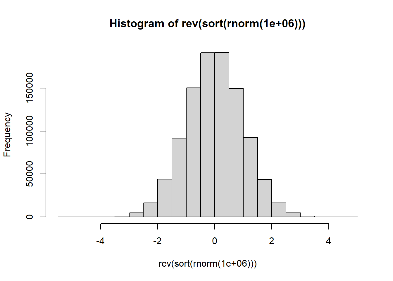

#>    user  system elapsed 
#>    0.17    0.00    0.18

Note that user and system times do not necessarily add up to elapsed time exactly.

Write the necessary code using proc.time() directly to obtain the execution time of hist (rev (sort (rnorm (1000000)))).
As an application of system.time() and proc.time() perform the following simulation study: Given a covariance matrix \(\mathbf{S}:p \times p\) the task is to compute the corresponding correlation matrix. The execution times of the following three methods are to be compared:
1. Direct elementwise calculation of \(r_{ij} = \frac{s_{ij}}{\sqrt{s_{ii}s_{jj}}}\) using two nested for loops;
2. Two applications of sweep();
3. Matrix multiplication where \(\mathbf{R}:p \times p = [diag(\mathbf{S})]^{-\frac{1}{2}} \mathbf{S} [diag(\mathbf{S})]^{-\frac{1}{2}}\) where \(diag(\mathbf{A})\) denotes the diagonal matrix formed from \(\mathbf{A}:p \times p\) by setting all its off-diagonal elements equal to zero.

Use var() and rnorm() to compute covariance matrices of different sizes \(p\) from samples varying in size \(n\). Study the role of \(n\) and \(p\) in the effectiveness (economy in execution time) of the above three methods. Display the results graphically. Remember that for valid comparisons the three methods must be executed with identical samples.

8.8 The calling of functions with argument lists

The function do.call() provides an alternative to the usual method of calling functions by name. It allows specifying the name of the function with its arguments in the form of a list:

mean ( c (1:100, 500), trim=0.1)
#> [1] 51
do.call ("mean", list( c (1:100, 500), trim=0.1))
#> [1] 51

How does do.call() differ from the function call()?
As an illustration of the usage of do.call() study the following example:

na.pattern <- function(frame)
{ nas <- is.na (frame)
  storage.mode (nas) <- "integer"
  table (do.call ("paste", c(as.data.frame(nas), sep = "")))
}
na.pattern(as.data.frame(airquality))
#> 
#> 000000 010000 100000 110000 
#>    111      5     35      2

What can be learned from the above output?

What is the difference between as.integer(), storage.mode() <– "integer", storage.mode() and mode()?

8.9 Evaluating R strings a commands

Recall from Figure 7.1 that the function parse(text = "3 + 4") returns the unevaluated expression 3 + 4. In order to evaluate the expression use function eval(): eval (parse (text = "3 + 4")) returns 7.

8.10 Object oriented programming in R

Suppose we would like to investigate the body of function plot(). We know that this can be done by entering the function’s name at the R prompt:

plot
#> function (x, y, ...) 
#> UseMethod("plot")
#> <bytecode: 0x00000163762b0f90>
#> <environment: namespace:base>

The presence of UseMethod("plot") shows that plot() is a generic function. The class of an object determines how it will be treated by a generic function i.e. what method will be applied to it. Function setClass() is used for setting the class attribute of an object. Function methods() is used to find out (a) what is the repertoire of methods of a generic function and (b) what methods are available for a certain class:

methods(plot) # repertoire of methods for FUNCTION plot()
#>  [1] plot.acf*           plot.data.frame*   
#>  [3] plot.decomposed.ts* plot.default       
#>  [5] plot.dendrogram*    plot.density*      
#>  [7] plot.ecdf           plot.factor*       
#>  [9] plot.formula*       plot.function      
#> [11] plot.hclust*        plot.histogram*    
#> [13] plot.HoltWinters*   plot.isoreg*       
#> [15] plot.lm*            plot.medpolish*    
#> [17] plot.mlm*           plot.ppr*          
#> [19] plot.prcomp*        plot.princomp*     
#> [21] plot.profile*       plot.profile.nls*  
#> [23] plot.R6*            plot.raster*       
#> [25] plot.spec*          plot.stepfun       
#> [27] plot.stl*           plot.table*        
#> [29] plot.ts             plot.tskernel*     
#> [31] plot.TukeyHSD*     
#> see '?methods' for accessing help and source code
methods(class="lm")  # what methods are available for CLASS lm
#>  [1] add1           alias          anova         
#>  [4] case.names     coerce         confint       
#>  [7] cooks.distance deviance       dfbeta        
#> [10] dfbetas        drop1          dummy.coef    
#> [13] effects        extractAIC     family        
#> [16] formula        hatvalues      influence     
#> [19] initialize     kappa          labels        
#> [22] logLik         model.frame    model.matrix  
#> [25] nobs           plot           predict       
#> [28] print          proj           qr            
#> [31] residuals      rstandard      rstudent      
#> [34] show           simulate       slotsFromS3   
#> [37] summary        variable.names vcov          
#> see '?methods' for accessing help and source code

In broad terms there are currently three types of classes in use in R: The old classes or S3 classes and the newer S4 and S5 (also called reference classes) classes. The newer classes can contain one or more slots which can be accessed using the operator @. Central to the concept of object oriented programming is that a method can inherit from another method. The function NextMethod() provides a mechanism for inheritance.

As an example of a generic function study the example in the help file of the function all.equal().
R provides many more facilities for writing object oriented functions. Consult the R Language Definition Manual Chapter 5: Object-Oriented Programming for further details.
A statistical investigation is often concerned with survey or questionnaire data where respondents must select one of several categorical alternatives. The questdata below shows the responses made by 10 respondents on four questions. The alternatives for each question were measured on a five point categorical scale. We can refer to the questdata dataframe as the full data. This form of representing the data is not an effective way of storing the data when the number of respondents is large. A more compact way of saving the data without any loss in information is to store the data in the form of a response pattern matrix or dataframe. The first row of questdata constitutes one particular response pattern namely ("b" "c" "a" "d"). A response pattern matrix (dataframe) shows all the unique response patterns together with the frequency with which each of the different response patterns has occurred. Your challenge is to provide the necessary R functions to convert the full data into a response pattern representation, and conversely to recover the full data from its response pattern representation.

questdata <- rbind (c("b", "c", "a", "d"),
                    c("d", "d", "c", "a"),
                    c("a", "d", "c", "e"),
                    c("a", "d", "c", "e"),
                    c("b", "c", "a", "d"),
                    c("a", "d", "c", "e"),
                    c("b", "c", "a", "d"),
                    c("d", "d", "c", "a"),
                    c("c", "b", "a", "e"),
                    c("b", "c", "a", "d"))
colnames(questdata) <- c("Q1", "Q2", "Q3", "Q4")

Create the R object questdata and then give the following instructions:

unique (questdata [,1])
#> [1] "b" "d" "a" "c"
duplicated (questdata)
#>  [1] FALSE FALSE FALSE  TRUE  TRUE  TRUE  TRUE  TRUE FALSE
#> [10]  TRUE
duplicated (questdata, MARGIN = 1)
#>  [1] FALSE FALSE FALSE  TRUE  TRUE  TRUE  TRUE  TRUE FALSE
#> [10]  TRUE
duplicated (questdata, MARGIN = 2)
#>    Q1    Q2    Q3    Q4 
#> FALSE FALSE FALSE FALSE
unique (questdata)
#>      Q1  Q2  Q3  Q4 
#> [1,] "b" "c" "a" "d"
#> [2,] "d" "d" "c" "a"
#> [3,] "a" "d" "c" "e"
#> [4,] "c" "b" "a" "e"
unique (questdata, MARGIN = 1)
#>      Q1  Q2  Q3  Q4 
#> [1,] "b" "c" "a" "d"
#> [2,] "d" "d" "c" "a"
#> [3,] "a" "d" "c" "e"
#> [4,] "c" "b" "a" "e"
unique (questdata, MARGIN = 2)
#>       Q1  Q2  Q3  Q4 
#>  [1,] "b" "c" "a" "d"
#>  [2,] "d" "d" "c" "a"
#>  [3,] "a" "d" "c" "e"
#>  [4,] "a" "d" "c" "e"
#>  [5,] "b" "c" "a" "d"
#>  [6,] "a" "d" "c" "e"
#>  [7,] "b" "c" "a" "d"
#>  [8,] "d" "d" "c" "a"
#>  [9,] "c" "b" "a" "e"
#> [10,] "b" "c" "a" "d"

Examine Table 3.5 and carefully describe the behaviour of the functions duplicated() and unique().

Write an R function, say full2resp to obtain the response pattern representation of questionnaire data like those given above. Test your function on questdata.
Write an R function, say resp2full to obtain the full data set given its response pattern representation. Test your function on the response pattern representation of the questdata.

8.11 Recursion

Functions in R can call themselves. This process is called recursion and it is implemented in R programming by the function Recall().

As an example we will use recursion to calculate \(x(x+1)(x+2)\dots(x+k)\) with \(k\) a positive integer:

recurs.example <- function (x, k) 
{ # Function to calculate x(x+1)(x+2).....(x+k)
  # where k is a positive integer.
     if (k < 0 ) 
      stop("k not allowed to be negative or non-integer")
    else if( k == 0) x
       else(x+k) * Recall(x,k-1)
   }

Investigate if recurs.example() works correctly.

Explain how recursion works by studying the output of the following function for values of \(r = 1, 2, 3, 4, 5, 6\):

Recursiontest <- function (r)
{ if (r <= 0) NULL
  else { cat("Write = ", r, "\n")
         Recall (r - 1)
         Recall (r - 2)
       }
}
Recursiontest(1)
#> Write =  1
#> NULL
Recursiontest(2)
#> Write =  2 
#> Write =  1
#> NULL
Recursiontest(3)
#> Write =  3 
#> Write =  2 
#> Write =  1 
#> Write =  1
#> NULL
Recursiontest(4)
#> Write =  4 
#> Write =  3 
#> Write =  2 
#> Write =  1 
#> Write =  1 
#> Write =  2 
#> Write =  1
#> NULL
Recursiontest(5)
#> Write =  5 
#> Write =  4 
#> Write =  3 
#> Write =  2 
#> Write =  1 
#> Write =  1 
#> Write =  2 
#> Write =  1 
#> Write =  3 
#> Write =  2 
#> Write =  1 
#> Write =  1
#> NULL
Recursiontest(6)
#> Write =  6 
#> Write =  5 
#> Write =  4 
#> Write =  3 
#> Write =  2 
#> Write =  1 
#> Write =  1 
#> Write =  2 
#> Write =  1 
#> Write =  3 
#> Write =  2 
#> Write =  1 
#> Write =  1 
#> Write =  4 
#> Write =  3 
#> Write =  2 
#> Write =  1 
#> Write =  1 
#> Write =  2 
#> Write =  1
#> NULL

Use recursion and the function Recall() to write an R function to calculate \(x!\).
Use recursion to write an R function that generates a matrix whose rows contain subsets of size \(r\) of the first \(n\) elements of the vector v. Ignore the possibility of repeated values in v and give this vector the default value of 1:n.

8.12 Environments in R

Study the following parts from the R Language definition Manual: § 3.5 Scope of variables; Chapter 4: Functions.

Consider an R function xx(argument). Write an R function to add a constant to the correct object (i.e. the object in the correct environment) that corresponds to argument. In order to answer this question, you must determine in which environment argument exists and evaluation must take place in this environment. Possible candidates to consider are the parent frame, the global environment and the search list. Assume that only the first data basis on the search list is not read-only so that in cases where argument can be found anywhere in the search list it can be assigned to the first data basis. Hint: Study how the following functions work: assign(), deparse(), invisible(), exists(), substitute(), sys.parent().

8.13 “Computing on the language”

Read R Language Definition Manual Chapter 6: Computing on the language.

8.14 Writing user friendly applications: the package shiny

The shiny package in R allows one to create an interactive environment inside R. As an example, the code below generates data from a bivariate normal distribution and makes a scatter plot of the two variables. With shiny a sliding bar is added where the user can adjust the correlation between the two variables.

A shiny app consists of a user interface (ui) a server function and the shinyApp function that uses the ui object and the server function to build a Shiny app object. For the sliding bar, the function sliderInput() is used. Table 8.1 provides a list of different input elements.

The server function uses the inputs – the cor.val in this example – to produce an output – the scatter plot in this example – using a reactive expression – the plot command in this example. The server function and thus the reactive expression is called with every change in the input, i.e. the plot is executed with the updated cor.val. The output produced by die server function – scatter in this example – is plotted in the mainPanel with the function plotOutput.

Table 8.1: Input elements for shiny apps.
`actionButton()`	`fileInput()`	`sliderInput()`
`checkboxGroupInput()`	`numericInput()`	`submitButton()`
`checkboxInput()`	`passwordInput()`	`textAreaInput()`
`dateInput()`	`radioButtons()`	`textInput()`
`dateRangeInput()`	`selectInput()`	`varSelectInput()`

library(shiny)

ui <- pageWithSidebar(
      headerPanel("Bivariate normal plot"),
      # App title

      sidebarPanel(
      # Sidebar panel for inputs

          sliderInput(inputId = "cor.val",
                      label = "Correlation",
                      min = -1,
                      max = 1,
                      value = 0,
                      step = 0.01
          )
      ),

      mainPanel(
      # Main panel for scatter plot

          textOutput("caption"),
          plotOutput("scatter")
      )
   )

server <- function(input, output) {
         require(MASS)
         sigma <- diag(2)

         output$caption <- renderText({ paste ("Bivariate normal data with 
                                correlation", input$cor.val)
                           })
         output$scatter <- renderPlot({  
                              sigma[1,2] <- sigma[2,1] <- input$cor.val
                              X <- mvrnorm(1000, mu=c(0,0), sigma)
                              plot(X,asp=1,col="red",pch=15)
                           })
      }

shinyApp(ui, server)

Adjust the shiny app above by adding three more input sources:

The number of observations to be generated.
Selecting the mean vector for the bivariate normal from the following options

\(\mathbf{\mu}' = [0, 0]\)
\(\mathbf{\mu}' = [10, 2]\)
\(\mathbf{\mu}' = [-3, -3]\)
\(\mathbf{\mu}' = [8, 207]\)

Having a series of radio buttons to choose the colour for the observations in the plot.

8.15 Exercise

Write an R function to determine which positive whole number elements \(≤10^{10}\) of a given vector are prime and to return these primes. Test this function with randomly generated vectors.
Repeat (a) using recursion.
Write a Shiny App that allows the user to choose between one of the data sets:LifeCycleSavings and state.x77 as a data matrix \(\mathbf{X}:n \times p\). The unweighted Minkowski metric for the pairwise distance between observation \(i\) and observation \(j\) is defined as \(d_{ij} = \left( \sum_{k=1}^p{|x_{ik}-x_{jk}|^λ} \right)^{(1/λ)}\), \(λ≥1\). Make provision for the user to choose the value of \(\lambda\) to be used to calculate the pairwise distances between all the rows of the data matrix. Note that \(λ=1\) is the Manhattan distance and \(λ=2\) is the Euclidean distance. Use \(λ=2\) as your default value.

8.16 The function on.exit()

What does the function on.exit() do?

One use of the special argument ... together with the on.exit() function is to allow a user to make temporary changes to graphical parameters of a graphical display within a function. This can be done as follows:

function(...)
 { oldpar <- par(...)
   on.exit(par(oldpar))  
   or on.exit(par(c(par(oldpar),par(mfrow = c(1,1)))))
   new plot instructions
   ..............................
  }

In the above it is assumed that only arguments of par() can be substituted when the function concerned is called. A further use of on.exit() is for temporarily changing options.

8.17 Error tracing

Any error that is generated during the execution of a function will record details of the calls that were being executed at the time. These details can be shown by using the function traceback(). The function dump.frames() gives more detailed information, but it must be used sparingly because it can create very large objects in the workspace. The function options (error = xx) can be used to specify the action taken when an error occurs. The recommended option during program development is options(error = recover). This ensures that an error during an interactive session will call recover() from the lowest relevant function call, usually the call that produced the error. You can then browse in this or any of the currently active calls to recover arbitrary information about the state of computation at the time of the error. An alternative is to set options(error = dump.frames). This will save all the data in the calls that were active when an error occurred. Calling debugger() later on produce a similar result to recover().

The following is a summary of the most common error tracing facilities in R:

Table 8.2: Error tracing facilities.
`print()`, `cat()`	The printing of key values within a function is often all that is needed.
`traceback()`	Must be used together with `dump.frames()`.
`options(warn=2)`	Changes warning to an error that causes a dump.
`options(error=)`	Changes the function that is used for the dump action.
`last.dump()`	The object in the .RData that contains a list of calls to dump.
`debugger()`	Function to inspect last.dump for an error.
`browser()`	Function that can be used within a function to interrupt the latter’s execution so that variables within the local frame concerned can be inspected.
`trace()`	Places tracing information before or within functions. Can be used to place calls to the browser at given positions within a function.
`untrace()`	Switches all or some of the functions of `trace()` off.

Study the R Language Manual Definition Chapter 9: Debugging for a summary of error tracing facilities in R . Note especially how the functions print(), cat(), traceback(), browser(), trace(), untrace(), debug(), undebug() and options(warn=2 or error=) work.
Study usage of: options(error = dump.frames); debugger()
Study usage of: options(error = dump.frames)
Study usage of the objects last.dump and .Traceback.

8.18 Error handling: The function `try()`

As an example of the need to be able to handle errors properly consider a simulation study involving a large number of repetitive calculations.

Example.8.18.a <- function (iter = 500)
{ select.sample <- function (x) 
  { temp <- rnorm (100, m = 50, s = 20)
    if (any (temp < 0)) stop("Negative numbers not allowed")
    mean(log(temp))                                                         }
  out <- lapply(1:iter, function(i) select.sample(i))
  out
}

With iter set to a large value, inevitably a call to Example.8.18.a() will result in an error message:

> Example.8.18.a()
Error in select.sample(i) : Negative numbers not allowed.

To see how try() can be used make the following change in Example.8.18.a():

Example.8.18.b <- function (iter = 500)
{ select.sample <- function (x) 
  { temp <- rnorm (100, m = 50, s = 20)
    if (any (temp < 0)) stop("Negative numbers not allowed")
    mean(log(temp))                                                         }
  out <- lapply(1:iter, function(i) 
                        try(select.sample(i), silent = TRUE))
  out
}

A typical chunk of output from a call to Example.8.18.b() is

> Example.8.18.b(2)
[[1]]
[1] 3.804975
[[2]]
[1] "Error in select.sample(i) : Negative numbers not allowed\n"
attr(,"class")
[1] "try-error"
attr(,"condition")
<simpleError in select.sample(i): Negative numbers not allowed>

Notice that execution of Example.8.18.b was not halted prematurely. From the above output we can make some final changes to our example function:

Example.8.18.c <- function (iter = 500)
{ select.sample <- function (x) 
  { temp <- rnorm (100, m = 50, s = 20)
    if (any (temp < 0)) stop("Negative numbers not allowed")
    mean(log(temp))                                                         }
  out <- lapply(1:iter, function(i) 
                        try(select.sample(i), silent = TRUE))
  out <- lapply(out, function(x)
                     { if (is.null (attr (x,"condition"))) x <- x
                       else x <- attr(x, "condition")
                     })
  Error.report <- lapply(out, function(x) 
                              ifelse(!is.numeric(x), x, "No Error"))
  Numeric.results <- unlist(lapply(out, function(x)   
                                        ifelse (is.numeric(x), x, NA)))
  list (Error.report = Error.report, Numeric.results = Numeric.results) 
}

Study the output of a call to Example.8.18.c and comment on the merits of try() in this example.

7 Writing functions in R

9 Reading data files into R, formatting and printing