3 R operators and functions
After completing Chapters 1 and 2 it is assumed that the following are now familiar:
- How to communicate with R;
- How to manage workspaces;
- How to perform simple tasks using R.
In this chapter we take a closer look at the behaviour of some of the most common
- R operators
- R functions.
3.1 Arithmetic operators
- Study the use of the operators in Table 3.1.
| Operator | Function | Operator | Function |
|---|---|---|---|
+ |
Addition | ^ |
Exponentiation |
- |
Subtraction | %/% |
Integer divide |
* |
Multiplication | %% |
Modulus |
/ |
Division | : |
Sequence |
%*% |
Matrix multiplication | - |
Uniry minus |
Note that the arithmetic operators are also functions. That this is so follows by studying the following examples:
3+7
#> [1] 10
"+"(3,7)
#> [1] 10
17 %% 3
#> [1] 2
"%%"(17,3)
#> [1] 2- Rules for operator expressions with vector arguments.
Study the results of the following R instructions.
cars [,2] * 12 * 25.4 / 1000
#>  [1]  0.6096  3.0480  1.2192  6.7056  4.8768  3.0480  5.4864
#>  [8]  7.9248 10.3632  5.1816  8.5344  4.2672  6.0960  7.3152
#> [15]  8.5344  7.9248 10.3632 10.3632 14.0208  7.9248 10.9728
#> [22] 18.2880 24.3840  6.0960  7.9248 16.4592  9.7536 12.1920
#> [29]  9.7536 12.1920 15.2400 12.8016 17.0688 23.1648 25.6032
#> [36] 10.9728 14.0208 20.7264  9.7536 14.6304 15.8496 17.0688
#> [43] 19.5072 20.1168 16.4592 21.3360 28.0416 28.3464 36.5760
#> [50] 25.9080
7%/%3
#> [1] 2
7%%3
#> [1] 1
matrix(1,nrow=4,ncol=4) * matrix(3,nrow=4,ncol=4)
#>      [,1] [,2] [,3] [,4]
#> [1,]    3    3    3    3
#> [2,]    3    3    3    3
#> [3,]    3    3    3    3
#> [4,]    3    3    3    3
matrix(1,nrow=4,ncol=4) %*% matrix(3,nrow=4,ncol=4)
#>      [,1] [,2] [,3] [,4]
#> [1,]   12   12   12   12
#> [2,]   12   12   12   12
#> [3,]   12   12   12   12
#> [4,]   12   12   12   12
Explain the following instructions and output from R:
1:12 + 1:3
#>  [1]  2  4  6  5  7  9  8 10 12 11 13 15
1:10 + 1:2
#>  [1]  2  4  4  6  6  8  8 10 10 12
1:10 + 1:3
#> Warning in 1:10 + 1:3: longer object length is not a
#> multiple of shorter object length
#>  [1]  2  4  6  5  7  9  8 10 12 11
In the above examples it is illustrated that R uses vectorized arithmetic i.e. it operates on vectors as wholes. Sometimes the recycling principle is applied with or without a warning. It is a good R programming habit to make use of vectorizing calculations where possible. The effect of the recycling principle must be kept in mind since it might lead to unwanted results.
- Missing values, infinity and “not a number”.
A missing value in R is denoted by NA. The result of a computation involving NAs is always NA e.g.
The result of a computation that cannot be represented as a number e.g. 0/0 is denoted by NaN.
Note: some computational results are differently reported by R as the corresponding algebraic equivalents, 5/0 in R is given by Inf while algebraically it is undefined.
- Scientific notation
R uses decimal notation as well as scientific notation for arithmetic calculations. Scientific notation is not to be confused with \(exp()\).
60000000
#> [1] 6e+07
1/6000000
#> [1] 1.666667e-07
exp(15)
#> [1] 3269017
exp(-15)
#> [1] 3.059023e-07- How are numbers represented in a computer’s memory? What are the implications of this?
Computers use ON/OFF (or 1/0) switches for encoding information. A single switch is called a bit and a group of eight bits is called a byte. A single integer is represented exactly in a computer by a fixed number of bytes i.e. 32 or 64 bits. There are several schemes according to which integers are represented by bits in a computer. This representation in a computer takes place at a level where R has no control over it but R stores information about the computing environment in an object .Machine. The element .Machine$integer.max returns the largest integer that can be represented in the computer on which R is running e.g.
.Machine$integer.max
#> [1] 2147483647
Although the above method of representing integers by strings of bits provides a very efficient way of storing integers in a computer R usually treats integers similar to real numbers by using floating point representation. In binary floating point notation a number x is written as a sequence of zeros and ones (the mantissa) times two with an exponent say \(m\): \(x=b_0 b_1 b_2…×2^m\) where \(b_0=1\) except when \(x=0\).
In practice there is only a limited number of \(b\)’s available and the exponent is also limited therefore, in general, not all real numbers can be represented exactly in a computer – they can at most be approximated. The smallest number \(x\) such that \(1 + x\) can be distinguished from \(1\) in a computer is called machine epsilon. In R this can be obtained from .Machine$double.eps e.g.
.Machine$double.eps
#> [1] 2.220446e-16
Although floating point representation allows computation with very small (in magnitude) and very large numbers the above limitations can lead to underflow or overflow which can have disastrous consequences in practice. Writing good code in R must take the above seriously into account.
3.2 Logical operators
Logical operators result in TRUE, FALSE or NA. Study the use of the logical operators in Table 3.2. Warning: While it is perfectly legitimate to write
x[x == -1] <- 0
x[x == 1] <- 0
it is incorrect to specify
The correct code in the latter case is
What are the consequences of the above code? Also take note of the functions any() and all(). These two functions are useful when combining logical objects. Give the necessary instructions to carry out the following tasks:
- Check which (if any) of the states in the
state.x77data set have populations with an illiteracy rate that is not larger than \(1.6\) and a Murder rate of more than \(10.0\). - Check if there is at least one state with income greater than \(\$5000\) and life expectancy less than \(70.0\) years.
- Check if all states with an income of more than \(\$5000\) has an illiteracy of below \(2.0\).
What is meant by a control logical operator?
| Operator | Function |
|---|---|
> |
Greater than |
< |
Less than |
<= |
Less than or equal to |
>= |
Greater than or equal to |
== |
Equality |
& |
Elementwise and |
| |
Elementwise or |
&& |
Control and |
|| |
Control or |
! |
Unary not |
!= |
Not equal to |
- Carry out the instructions:
mata <- matrix(1:4, ncol = 2)
matb <- matrix(c(10, 20, 30, 40), ncol = 2)
mata
#>      [,1] [,2]
#> [1,]    1    3
#> [2,]    2    4
matb
#>      [,1] [,2]
#> [1,]   10   30
#> [2,]   20   40
mata>1 & matb>1
#>       [,1] [,2]
#> [1,] FALSE TRUE
#> [2,]  TRUE TRUE
mata>1 | matb>1
#>      [,1] [,2]
#> [1,] TRUE TRUE
#> [2,] TRUE TRUE
mata>1 && matb>1
#> Error in mata > 1 && matb > 1: 'length = 4' in coercion to 'logical(1)'
mata>1 || matb>1
#> Error in mata > 1 || matb > 1: 'length = 4' in coercion to 'logical(1)'
Comment on the above.
- What is the result of
sum(c(TRUE, !FALSE, FALSE, TRUE, TRUE))? - What is the result of
sum(c(TRUE, !FALSE, FALSE, NA, TRUE))?
Explain
3.3 The operators <-, <<- and ~
Before considering the use of these operators answer the following:
What will happen to an object
aain the working directory if within a function the following assignment is madeaa <- 20?Now, study the help file of
<<-and then answer (a) if the operator<-has been replaced with the operator<<-. Warning: use<<-very carefully.The tilde operator is used in modelling functions, e.g.
lm (length ~ age).
3.4 Operator precedence
Study the precedence rules as summarized in Table 3.4.1. The rules followed are shown in Table 3.3 from top to bottom and left to right. Note the use of
- parentheses
( )for function arguments and changing precedence, - braces
{ }for demarcating blocks of instructions - and brackets
[ ]for subscripting.
The correct way of extracting the fifth element of a sequence like 1:20 is
(1:20)[5]
#> [1] 5| Operator | What it does |
|---|---|
$ |
List and dataframe subscripting |
[], [[]]
|
Vector and matrix subscripting; list subscripting |
^ |
Exponentiation |
%*%, %/%, %%
|
Matrix multiplication; integer divide; modulus |
*, /
|
Multiplication and division |
+, -
|
Addition and subtraction |
<, >, <=, >=, ==, !=
|
Logical comparisons |
! |
Unary not |
&, |, &&, ||
|
Logical and; logical or; control and; control or |
<-, <<-
|
Assignment |
Explain the result of the following R instructions:
20 / 4 * 12 ^2 - 6 + 1
#> [1] 715
(20 / 4) * (12 ^2) + (-6 + 14)
#> [1] 728
20 / 4 * 12 ^(2 - 6 + 14)
#> [1] 309586821120
20 / 4 * (12 ^2 - 6 + 14)
#> [1] 760
3.5 Some mathematical functions
3.5.1 General mathematical functions
abs(), exp(), log(x, base = exp(1)), log10(), gamma(), sign(), sqrt()
3.5.2 Trigonometric functions
See Table 3.4.
| Operator | Function | Operator | |
|---|---|---|---|
cos() |
cosine | acos() |
arc cosine |
sin() |
sine | asin() |
arc sine |
tan() |
tangent | atan() |
arc tangent |
cosh() |
hyperbolic cosine | acosh() |
arc hyperbolic cosine |
sinh() |
hyperbolic sine | asinh() |
arc hyperbolic sine |
tanh() |
hyperbolic tangent | atanh() |
arc hyperbolic tangent |
3.5.4 Functions for rounding and truncating
round(), ceiling(), floor(), trunc()
Study the help files of the above functions. Check all arguments.
3.5.5 Functions for matrices
Study Table 3.5 in detail.
Two other functions that play an important role in matrix calculations are the functions rbind() and cbind() for concatenating matrices row-wise or column-wise. Also revise the functions matrix(), dim(), dimnames(), colnames(), rownames() as well as scan() and read.table().
| Function | What it does |
|---|---|
chol() |
Cholesky decomposition |
crossprod() |
Matrix crossproduct |
diag() |
Create identity matrix, diagonal matrix or extract diagonal elements depending on its argument |
eigen() |
Finding eigenvectors and eigenvalues |
kronecker() |
Computing the kronecker product of two matrices |
outer() |
Outer product of two vectors |
scale() |
Centring and scaling a data matrix |
solve() |
Finding the inverse of a nonsingular matrix |
svd() |
Singular value decomposition of a rectangular matrix |
qr() |
QR orthogonalization |
t() |
Transpose of a matrix |
The function
chol()performs a Cholesky decomposition of the square, symmetric, positive definite matrix \(\mathbf{A}=\mathbf{U}'\mathbf{U}\) where \(\mathbf{U}\) is an upper triangular matrix.The function
crossprod (A, B)returns the matrix \(\mathbf{A'B}\).The function
diag(arg)performs various actions depending on its argument: ifargis a positive integerdiag(arg)returns an identity matrix of the given size; ifargis a vectordiag(arg)returns a diagonal matrix with diagonal elements the respective elements of the given vector; ifargis a matrix thendiag(arg)returns a vector containing the diagonal elements of the given matrix.What is the difference between
diag(A)anddiag(diag(A))whereAis a square matrix?The function
eigen()operates on a square matrix and returns a list with named elementsvaluesandvectorscontaining respectively, the eigenvalues and eigenvectors. Study the help file ofeigen()carefully.The function
kronecker()returns the Kronecker product \(\mathbf{A} \otimes \mathbf{B}\) of matrices \(\mathbf{A}\) and \(\mathbf{B}\).The function
outer (x, y, f)operates on two vectors \(x:n\times 1\) and \(y:p\times 1\) to return a matrix of size \(n \times p\) with \(ij\)th element the result of applying the functionfonx[i]andy[j]. The default forfis*.The function
scale()has three arguments: a matrix as first argument; a second argumentcenterand a third argumentscale. Ifcenter = FALSE, no centring of the columns of the matrix argument is performed, if set toTRUE(the default), the mean value of each column is subtracted from the respective columns, if given a vector of values these values are subtracted from the respective columns. Ifscale = FALSE, no scaling of the columns of the matrix argument is performed, if set toTRUE(the default) each column is divided by its standard deviation, if given a vector of values then each column is divided by the corresponding value.The function
solve (A, b)is used for solving the equation \(\mathbf{Ax=b}\) for \(\mathbf{x}\), where \(\mathbf{b}\) can be either a vector or a matrix with \(\mathbf{A}\) being a square matrix. If argumentbis missing it is taken to be the identity matrix so that the inverse of argumentAis returned.The function
svd()returns the singular value decomposition of its matrix argument \(\mathbf{A=UDV}'\). It returns a list with three components:uthe orthogonal or orthonormal matrix \(\mathbf{U}\);dthe vector containing the ordered singular values of the rectangular matrix \(\mathbf{A}\);vthe orthogonal or orthonormal matrix \(\mathbf{V}\).The function
qr()performs a QR decomposition of any arbitrary matrix \(\mathbf{M=QR}\) with \(\mathbf{Q}\) and orthogonal matrix and \(\mathbf{R}\) an upper triangular matrix. Study the help file ofqr()for full details and usages of the function. Note that the matrices \(\mathbf{Q}\) and \(\mathbf{R}\) can be obtained directly by callingqr.Q(qr())andqr.R(qr()), respectively.
- What is the meaning of each of the following instructions?
rbind(a,b); rbind(1,x); rbind(a = 1:5,b = 10:14,c=20:24); cbind( a= 1:5, b=10:14, c=20:24)
Write a function to calculate the determinant of a square matrix. Name this function
det.own()in order to distinguish it from the built in R functiondet().When the user is satisfied with a function, it is often necessary to have it available for all R projects. It is useful to assign all such functions to the same data base or folder. Use the function
assign (x, object, pos = , envir = )to store the functiondet.own()in your own R functions folder. The argumentxinassign()is a character string for assigning a name to the object. The functionremove (list of objects names, pos = , envir = )can be used to remove objects from your own or any other database. Hint: First create a file and then useattach()to add it to the R search path.
Study how save() works.
Study how attach() works.
Study how assign() works.
Explain the use of the argument list=objects(2). To summarize: The construction NAME <- object is a simple way to assign an object to a name. This form of assignment always takes place in the global environment (the workspace). Assignment can also be performed using the functions save() and assign() as illustrated above. The latter form of assignment is more complicated but the assignment is not restricted to the global environment.
The result of the function
gamma(x)is \((x-1)!\) if \(x\) is a non-negative whole number. Now write a functionfact()to calculate \(x!\). This function must make provision for \(0!\) as well as for a negative number or a fraction that is read in by mistake. Hint: First study the usage of the if statement by requesting help?Control, recall Table 1.1. Store this function in your folder of R functions. How will you go about to makefact()anddet.own()available for any R project?The function
lgamma(x)returns the logarithms of \(\Gamma(x)\). Write a function to calculate the value of \(f(n) = \frac{\Gamma(\frac{n-1}{2})}{\Gamma(\frac{1}{2})\Gamma(\frac{n-2}{2})}\). Calculate the value of \(f(n)\) for \(n = -10, 10, 100, 500, 1000\).
3.5.6 Sorting functions
Note the use of the functions sort(), order() and rank(). First construct MatX using the functions scan() and matrix(). Explain in detail what order() does by sorting all the columns of MatX according to the values in the first column of the matrix.
\[ MatX = \begin{bmatrix} 4 & 80 & 12\\ 5 & 70 & 70\\ 6 & 30 & 19\\ 2 & 40 & 80\\ 4 & 90 & 40\\ 1 & 60 & 50\\ 7 & 10 & 20\\ 3 & 30 & 200 \end{bmatrix} \]
3.5.7 Some functions for data manipulation
Study the functions in Table 3.6.
| Function | What it does |
|---|---|
append() |
Combine vectors; more flexibility than c()
|
c() |
Create vectors |
duplicated() |
Extract duplicated values |
match() |
Match values in pairs of vectors |
pmatch() |
Partial matching |
replace() |
Replace specified values in vectors |
unique() |
Extract unique values |
Insert the vector (101, 102, 103, 104, 105) into the vector (10, 11, 12, 13, 14, 15, 16, 17, 18, 19, 20) after its fifth element by utilising the argument
afterof the functionappend().The function
replace()requires three argumentsx,listandvals. The values inxwith indices given inlistis replaced by the successive values invalsmaking use of the recycling principle if needed. Explain this by replacing in the vector (10, 2, 7, 20, 5, 8, 9, 20, 9, 1,1 15), the values 10, 20 and 15 with zeros.Find the unique values in the vector (10, 2, 7, 20, 5, 8, 9, 20, 9, 1, 15).
Find the duplicated values in the vector (10, 2, 7, 20, 5, 8, 9, 20, 9, 1, 15, 20, 20, 15).
Explain the usage of
match()by considering the difference between
3.5.8 Basic statistical functions
Study the functions in detail in Table 3.7.
| Function | What it does | Comments |
|---|---|---|
cor() |
Correlation | One or two arguments |
cumsum() |
Cumulative sum of elements of a vector | |
mean() |
Arithmetic mean | Optional argument trim =
|
median() |
Median | Accepts variable number of arguments |
min() |
Minimum value | Accepts variable number of arguments |
max() |
Maximum value | Accepts variable number of arguments |
prod() |
Product of elements of a vector | Accepts variable number of arguments |
cumprod() |
Cumulative product of elements of a vector | |
quantile() |
Returns specified quantiles | |
range() |
Minimum and maximum of a vector | Accepts variable number of arguments |
sample() |
Random sample | With or without replacement |
sum() |
Arithmetic sum | Also used for counting |
var() |
Variance and covariance; uses n-1 as denominator | Accepts vectors or matrices |
sd() |
Standard deviation; uses n-1 as denominator | Accept a vector as argument |
Note also the functions pmax() and pmin().
- Find the average Life Expectancy of the states in the
state.x77data set. - Find the 5% trimmed mean for Illiteracy of the states in the
state.x77data set. Hint:?meanprovides help for the functionmean(). - Find the correlation between the Illiteracy and the Income of the states in the
state.x77data set. - Find the covariance matrix of all the variables in the
state.x77data set. - Find the range for Murder in the
state.x77data set. - Obtain the details of a random sample of 10 states in the
state.x77data set. - Obtain two independent random permutations of the numbers \(1, 2, \dots, 10\).
- Write a function for computing the coefficient of kurtosis for a random sample. Test your function on the Frost variable in the
state.x77data set. - Write a function for computing the coefficient of skewness for a random sample. Test your function on the Murder variable in the
state.x77data set. - Write a function to compute the harmonic mean of a numeric vector. Test your function on the Life Expectancy of the states in the
state.x77data set. Compare your answer to your answer in (a).
3.5.9 Probability distributions in R
First, execute the R-instruction
help.search("distribution")to obtain a list of available statistical distributions in R. Each distribution has an identifying name preceded by one of the letters d, p, q or r. In the case of an F-distribution, for example, the identifier is just the letter f and for a normal distribution the identifier is norm. Preceding the distribution’s identifier by one of the letters d, p, q or r returns a density value, a probability, a quantile or a random sample for the specified distribution (probability density function or probability mass function). See Figure 3.1 for an explanation.
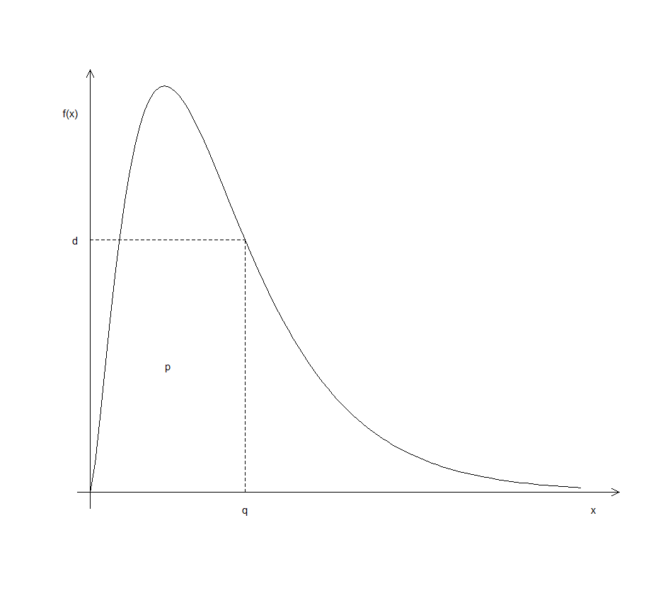
Figure 3.1: Meaning of the letters d, p and q when preceding an R distribution identifier.
3.5.10 Functions for categorical variables
Apart from being numeric or logical, data in R can also be categorical (factor in R) or character strings. Study in detail the functions operating on factor data in Table 3.8.
Use
cut()to create an objectareagrpto divide thestate.x77data set into three groups representing the states with area within the intervals \((0, 10 000]\),\((10 000, 100 000]\) and \((100 000, Inf]\), respectively. Hint: First study the arguments ofcut().Repeat (a) with argument
labels = ??to specify each state as being Small, Medium or Large with respect to its area.Use
unclass()to obtain the numeric codes associated with each level ofareagrp.Repeat (a) to obtain
areagrp2containing five equally spaced categories.Repeat (a) to obtain
areagrp3containing five groups with each containing \(20\%\) of the data.Use
cut()to create an objectillitgrpto divide thestate.x77data set into five groups representing the states with illiteracy within the interval \([0, 0.50)\), \([0.50, 1.00)\), \([1.00, 1.50)\), \([1.50, 2.00)\) and \([2.00, 5.00)\), respectively.Obtain a two-way table of the
state.x77data set according toareagrpandillitgrp.
| Function | What it does |
|---|---|
cut() |
Creates categories out of a continuous variable |
factor() |
Encodes a vector as a nominal categorical variable |
ordered() |
Encodes a vector as a ordinal categorical variable when argument ordered is set to TRUE |
levels() |
Displays or sets the levels of a factor variable |
pretty() |
Creates convenient break points for a categorical variable |
split() |
Breaks up an array according to the value of a categorical variable |
table() |
Counts the number of observations cross-classified by categories |
unclass() |
Returns the numeric codes for representing the levels of a factor variable |
3.5.11 Functions for character manipulation
Study the functions in Table 3.9 in detail.
| Function | What it does |
|---|---|
abbreviate() |
Generates abbreviations of character values |
cat() |
Display,messages and/or values on screen or send to file |
grep() |
Search for patterns in characters |
nchar() |
Number of characters in a string |
paste() |
Combine values into character strings |
strsplit() |
Split the elements of a character vector \(\times\) into substrings |
substring() |
Extracts parts of character strings |
What is the returned value of
grep ("ia", state.name)?Discuss the usage of
grep ("ia", state.name).Discuss the output of
objects (pos = grep("stats", search())).Use
paste()to create variable names: var1, var2, …, var100.Repeat (d) to create variable names: var_1, var_2, …, var_100.
Discuss the output of:
substring (paste (letters, collapse = ""),
             1:nchar (paste (letters, collapse="")),
1:nchar (paste (letters, collapse="")))- From the Help menu, select Manuals (in PDF) and open the Introduction to R document. Obtain a copy of the first two paragraphs of the Preface on page 1 of this book in the R commands window. Use this copy to calculate the number of words as well as the total number of characters (including spaces between words) in the passage.
We are going to use several of the functions in Table 3.9 to perform this task in steps. Proceed as follows in R after copying the relevant passage to the clipboard:
TextPar <- scan(file = "clipboard", what = "")To obtain a vector containing each of the words as a separate element.
TextPar <- paste (TextPar, collapse = " ")To convert TextPar into a vector containing one element consisting of all the words concatenated and separated by spaces into a single character string. Add the correct line breaks (“\n”) in TextPar using e.g. fix().
TextPar <- strsplit(x = TextPar, split = '\n')
TextPar <- unlist(TextPar)To change TextPar into a character vector.
3.6 Differentiation and integration
3.6.2 Integration
Study the help file of integrate().
3.6.3 Exercise
It is known from elementary statistics that approximately 68% of data from a normal distribution with a mean of zero and a standard deviation of unity will have an absolute value less than unity. Use the
sum()andrnorm()functions to find the proportion of \(n\) random \(normal (0, 1)\) variables whose absolute value is less than \(1.0\). Repeat with different values for \(n\) to investigate how widely the results vary.Define: conditional inverse and generalized (Moore-Penrose) inverse for matrix \(\mathbf{X}: p \times q\) and make provision for \(p = q\), \(p > q\) and \(p < q\). First, show how the svd of \(\mathbf{X}\) can be used to obtain a conditional inverse, \(\mathbf{X}^c\) for \(\mathbf{X}\). Now use the above information to write an R function for calculating \(\mathbf{X}^c\) for any given \(\mathbf{X}\). The function must provide a test to check if the calculated conditional inverse is indeed a conditional inverse. Illustrate the usage of your function.
-
Give the necessary instructions to:
- read into R an external text data file consisting of \(10\) sample observations with each consisting of one character variable and two numerical variables.
- read into R a large external text data file consisting of \(50\) numerical variables but unknown number of records. Each record in this data file takes up 5 lines. The variables in the R object must have the names X1, …, X50.
-
Discuss the meaning of the following R instructions:
y <- x[!is.na(x)]z <- (x + y)[!is.na(x) & x >0]a <- x[-(1:5)]x[is.na(x)] <- 0