7 Writing functions in R
Although we have already written various functions in R, in this chapter the writing of R functions will be approached systematically.
7.1 General
A good way to learn about functions or to write a new function is to look at existing ones. As an example consider that we would like to write a function to implement a novel plotting procedure. So we start by taking a look at the existing plot function.
plot
#> function (x, y, ...)
#> UseMethod("plot")
#> <bytecode: 0x000002ba86aa7770>
#> <environment: namespace:base>
This is not very helpful so we give the instruction:
methods(plot)
#>  [1] plot.acf*           plot.data.frame*
#>  [3] plot.decomposed.ts* plot.default
#>  [5] plot.dendrogram*    plot.density*
#>  [7] plot.ecdf           plot.factor*
#>  [9] plot.formula*       plot.function
#> [11] plot.hclust*        plot.histogram*
#> [13] plot.HoltWinters*   plot.isoreg*
#> [15] plot.lm*            plot.medpolish*
#> [17] plot.mlm*           plot.ppr*
#> [19] plot.prcomp*        plot.princomp*
#> [21] plot.profile*       plot.profile.nls*
#> [23] plot.R6*            plot.raster*
#> [25] plot.spec*          plot.stepfun
#> [27] plot.stl*           plot.table*
#> [29] plot.ts             plot.tskernel*
#> [31] plot.TukeyHSD*
#> see '?methods' for accessing help and source code
If we decide to take a look at plot.default we can do so by
plot.default
#> function (x, y = NULL, type = "p", xlim = NULL, ylim = NULL,
#>     log = "", main = NULL, sub = NULL, xlab = NULL, ylab = NULL,
#>     ann = par("ann"), axes = TRUE, frame.plot = axes, panel.first = NULL,
#>     panel.last = NULL, asp = NA, xgap.axis = NA, ygap.axis = NA,
#>     ...)
#> {
#>     localAxis <- function(..., col, bg, pch, cex, lty, lwd) Axis(...)
#>     localBox <- function(..., col, bg, pch, cex, lty, lwd) box(...)
#>     localWindow <- function(..., col, bg, pch, cex, lty, lwd) plot.window(...)
#>     localTitle <- function(..., col, bg, pch, cex, lty, lwd) title(...)
#>     xlabel <- if (!missing(x))
#>         deparse1(substitute(x))
#>     ylabel <- if (!missing(y))
#>         deparse1(substitute(y))
#>     xy <- xy.coords(x, y, xlabel, ylabel, log)
#>     if (is.null(xlab))
#>         xlab <- xy$xlab
#>     if (is.null(ylab))
#>         ylab <- xy$ylab
#>     if (is.null(xlim))
#>         xlim <- range(xy$x[is.finite(xy$x)])
#>     if (is.null(ylim))
#>         ylim <- range(xy$y[is.finite(xy$y)])
#>     dev.hold()
#>     on.exit(dev.flush())
#>     plot.new()
#>     localWindow(xlim, ylim, log, asp, ...)
#>     panel.first
#>     plot.xy(xy, type, ...)
#>     panel.last
#>     if (axes) {
#>         localAxis(if (is.null(y))
#>             xy$x
#>         else x, side = 1, gap.axis = xgap.axis, ...)
#>         localAxis(if (is.null(y))
#>             x
#>         else y, side = 2, gap.axis = ygap.axis, ...)
#>     }
#>     if (frame.plot)
#>         localBox(...)
#>     if (ann)
#>         localTitle(main = main, sub = sub, xlab = xlab, ylab = ylab,
#>             ...)
#>     invisible()
#> }
#> <bytecode: 0x000002ba86ea8510>
#> <environment: namespace:graphics>
Since our new plotting method is aimed at categorical data we decide rather to take a look at plot.factor. But this is an asterisked function and hence is not visible:
plot.factor
#> Error: object 'plot.factor' not found
Asterisked functions can be inspected using the following method:
getAnywhere(plot.factor)
#> A single object matching 'plot.factor' was found
#> It was found in the following places
#>   registered S3 method for plot from namespace graphics
#>   namespace:graphics
#> with value
#>
#> function (x, y, legend.text = NULL, ...)
#> {
#>     if (missing(y) || is.factor(y)) {
#>         dargs <- list(...)
#>         axisnames <- dargs$axes %||% if (!is.null(dargs$xaxt))
#>             dargs$xaxt != "n"
#>         else TRUE
#>     }
#>     if (missing(y)) {
#>         barplot(table(x), axisnames = axisnames, ...)
#>     }
#>     else if (is.factor(y)) {
#>         if (is.null(legend.text))
#>             spineplot(x, y, ...)
#>         else {
#>             args <- c(list(x = x, y = y), list(...))
#>             args$yaxlabels <- legend.text
#>             do.call("spineplot", args)
#>         }
#>     }
#>     else if (is.numeric(y))
#>         boxplot(y ~ x, ...)
#>     else NextMethod("plot")
#> }
#> <bytecode: 0x000002bb01958b28>
#> <environment: namespace:graphics>
How are default values assigned to arguments of functions?
What is the default behaviour of
plot.factor()?What tasks can be achieved with
pmatch()and what is understood by partial matching? What will happen ifplot.factor()is called with (i)legend.text = 'AA=Agecat'; (ii)leg = 'AA=Agecat'? Explain.Discuss the usage of
missing().Give an example of the usage of the function
stop(message= " ").Give an example of the usage of the function
warning(message= " ").What is the usage of the function
warnings()?Why can functions be called without specifying any arguments e.g.
q()?If the body of a function consists only of a single instruction it is not necessary to enclose it with braces.
The convention is to use the last evaluated statement as a function’s return value. If several objects are to be returned gather them in a list.
The function
return()with a single object or a list of objects is useful to interrupt a function at some intermediate stage and return an object or a list of objects at that particular stage. This is usually done when a function is under development.Sometimes there is no meaningful value to return e.g. when a function is written primarily to produce some plot. In cases like this the function
invisible()can be used as the last statement of the function. As an example of the usage ofinvisible()give the following instructions:
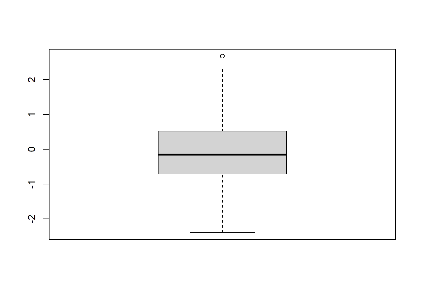
boxplot(rnorm(100), plot = FALSE)
#> $stats
#>            [,1]
#> [1,] -2.5860633
#> [2,] -0.8866465
#> [3,] -0.1002753
#> [4,]  0.4836419
#> [5,]  2.5049138
#>
#> $n
#> [1] 100
#>
#> $conf
#>            [,1]
#> [1,] -0.3167808
#> [2,]  0.1162303
#>
#> $out
#> numeric(0)
#>
#> $group
#> numeric(0)
#>
#> $names
#> [1] "1"
Now look at the end of function boxplot.default() to see how invisible() has been implemented.
Libraries (packages) of R functions. Attaching and detaching libraries to the search path. (Revise Chapter 1)
Creating a new function using scripts or
fix(). (Revise Chapter 1)Editing an existing function using scripts or
fix(). (Revise Chapter 1)Note that when writing a function a line can be interrupted at any place and be continued on a next line. Warning: Be careful not to put the break point where it marks the completion of an executable statement. Explain.
7.2 Writing a new function
Determining the indices of elements in a vector or matrix that meet a certain condition: the function where()
- Write the following function:
where <- function(x, cond)
{ # Argument cond must evaluate to a logical value
     if(!is.matrix(x))
       seq(along = x)[cond]
     else matrix(c(row(x)[cond], col(x)[cond]), ncol = 2)
}
Inspect the airquality data set using the command
str(airquality).Use the
where()function to find the indices of (i) theNAs, (ii) the maximum value and (iii) the minimum value in the airquality data set.Repeat (b) using the built-in function
which().
7.3 Checking for object name clashes
What happens if an R object is given the same name as an existing object?
Discuss the usages of the functions
apropos(),conflicts(),find()andmatch()for the naming of objects.Remember that when a function is called the R evaluator first looks in the global environment for a function with this name and subsequently in each of the attached packages or date bases in the order shown by
search(). The evaluator generally stops searching when the name is found for the first time. If two attached packages have functions with the same name one of them will mask the object in the other. For example, the functiongam()exists in two packages:gamandmgcv. If both were attached the command
library (mgcv)
#> Loading required package: nlme
#> This is mgcv 1.9-3. For overview type 'help("mgcv-package")'.
library (gam)
#> Loading required package: splines
#> Loading required package: foreach
#> Loaded gam 1.22-6
#>
#> Attaching package: 'gam'
#> The following objects are masked from 'package:mgcv':
#>
#>     gam, gam.control, gam.fit, s
find("gam")
#> [1] "package:gam"  "package:mgcv"
will return both version.
The operator
::can be used to access the intended version ofgam()by using the callmgcv::gam()orgam::gam().When writing R packages the namespace of the package provides another mechanism for ensuring that the correct version of a function is used. Note in this regard that the operator
:::can be used to access objects that are not exported.
7.4 Returning multiple values
7.4.1 Exercise
Write an R function that returns the mean, median, variance, minimum, maximum and coefficient of variation of a numeric vector of sample data. The different components must be accessible by name. Test your function with the value of rnorm(1000). Hint: Use the construct list (mean = ..., median = ..., ...).
7.5 Local variables and evaluation environments
Where is an object stored that is created by a script or
fix()?Where are local objects (objects that are created during the execution of a function) stored?
Explain how the evaluation environment works.
What is understood by the global environment?
Study the R help-file w.r.t. the operator
<<-. When is it useful to use this operator? What are the dangers inherent to this operator?What is understood by the scope of an expression or function?
The symbols which occur in the body of a function can be divided into three classes: formal parameters, local variables and free variables. The formal parameters of a function are those appearing within the parentheses denoting the argument list of the function. Their values are determined by the process of binding the actual function arguments to the formal parameters. Local variables are created by the evaluation of expressions in the body of the functions. Variables which are neither formal parameters nor local variables are called free variables. Free variables become local variables when they are assigned to. Consider the following function definition.
In this function, datvec is a formal parameter, the object mean on the left-hand of the assignment symbol is a local variable (not to be confused with the function mean() on the right-hand side of the assignment symbol) while Traffic is a free variable. In R the free variable bindings are resolved by first looking in the environment in which the function was created. This is called lexical scope.
If the following function call is made from the prompt in the working directory fun(1:25) the formal parameter datvec within the body of the function is assigned the value 1:25 (the actual argument) and its mean is assigned to the local object mean. If the free parameter Traffic is found in the global environment or in a data base on the search path the required graph will be created else an error message will be sent to the console. Perform the above call.
7.6 Cleaning up
Study how the function
on.exit()is used. This function can be used to reset options that are changed during an R-session back to their original values when the session is ended or a function terminates with an error message. It is also convenient for removal of temporary files.Study the uses of the functions
.First()and.Last().Write a function that automatically opens a graph window with a square plot region when an R-session is started.
7.7 Variable number of arguments: argument ...
- Consider the following situation: You want to write a function for a complex task. At a particular stage a graph of some intermediate results is to be constructed. This requires the calling function to contain a call to the
hist()function. Here is an example of a chunk of code for executing this task:
complexfun <- function(datmat,colgraph)
    { datmat <- scale(datmat)
       # Several lines of complex code here
      hist(datmat, col = colgraph)              }
A call like complexfun(rnorm(1000), 'yellow') can now be executed for the desired result. The problem is that the hist function has several arguments that you would like to be able to access by passing suitable actual values to them through the calling function complexfun. Instead of having to resort to provide a complete set of arguments in the argument list of complexfun R provides a neat way of addressing this situation: The argument ... which acts like any other formal argument except that it can represent a variable number of arguments. To see how the argument ... works change the above function to:
complexfun2 <- function(datmat, ... )
 { datmat <- scale(datmat)
       # Several lines of complex code here
   hist(datmat, ... )    }
Arguments represented by argument ... in the argument list of hist are passed to hist through the argument ... appearing in the arguments list of function complexfun2:
- Write a function that will retrieve the maximum length of any of an unspecified number of arguments of a specified mode. This is another example of the use of the
...argument:
maxlen <- function (mode.use="numeric", ...)
  { my.list <- list(...)
    out <- 0
    for(x in my.list)
      print (mode(x)) #if(mode(x) == mode.use) out <- max(out,length(x))
    out
  }
Note that the named argument must be specified as such in the function call:
maxlen(1:10, 1:15, 1:3, letters)
#> [1] "numeric"
#> [1] "numeric"
#> [1] "character"
#> [1] 0
maxlen(mode.use="numeric", 1:10, 1:15, 1:3, letters)
#> [1] "numeric"
#> [1] "numeric"
#> [1] "numeric"
#> [1] "character"
#> [1] 0
maxlen(1:10, 1:15, 1:3, letters, mode.use="character")
#> [1] "numeric"
#> [1] "numeric"
#> [1] "numeric"
#> [1] "character"
#> [1] 0
maxlen(mode.use="character", 1:10, 1:15, 1:3, letters)
#> [1] "numeric"
#> [1] "numeric"
#> [1] "numeric"
#> [1] "character"
#> [1] 0
7.8 Retrieving names of arguments: functions deparse() and substitute()
There are many practical situations requiring the conversion of mathematical expressions into character strings (text) or, conversely, requiring the conversion of text into mathematical expressions. The tools (functions) provided in R for achieving such conversions are summarized in Figure 7.1.
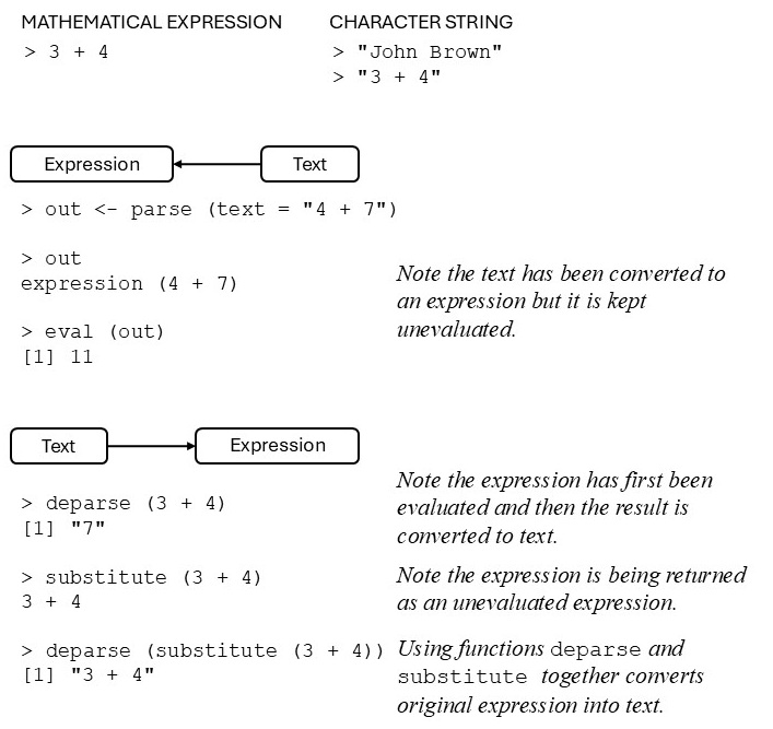
Figure 7.1: Converting text into mathematical expression or mathematical expressions into text.
- Task: write an R function that will plot two vectors using as axis labels the names of the objects passed as arguments to the function.
It follows from Figure 7.1 that the function substitute() takes an expression as argument and returns it unevaluated. In order to evaluate the return value of substitute() the function eval() must be used. The function deparse() takes as argument an unevaluated expression and converts it into a character string. Now we are ready to write the following function:
labplot <- function (x,y)
{ xname <- deparse(substitute(x))
 yname <- deparse(substitute(y))
 plot(x,y, xlab=xname, ylab=yname, main = paste("Plot of",
        yname,"versus", xname))
}7.9 Operators
Execute the following instruction
objects('package:base')[1:31]
#>  [1] "-"                 "-.Date"
#>  [3] "-.POSIXt"          "!"
#>  [5] "!.hexmode"         "!.octmode"
#>  [7] "!="                "$"
#>  [9] "$.DLLInfo"         "$.package_version"
#> [11] "$<-"               "$<-.data.frame"
#> [13] "$<-.POSIXlt"       "%%"
#> [15] "%*%"               "%/%"
#> [17] "%||%"              "%in%"
#> [19] "%o%"               "%x%"
#> [21] "&"                 "&&"
#> [23] "&.hexmode"         "&.octmode"
#> [25] "("                 "*"
#> [27] "*.difftime"        "/"
#> [29] "/.difftime"        ":"
#> [31] "::"
in order to obtain some examples of operators available in R.
- Operators are special R functions. Discuss this statement. In what respects do operators differ from ordinary R functions?
- Write an operator
%E%to determine the Euclidean distance between two vectors and give an example of its usage. Hint: when creating operators withfix()or using scripts the name must be given as a character string e.g.fix("%E%").
7.10 Replacement functions
Execute the following instruction
objects('package:base')[300:400]
#>   [1] "c.factor"
#>   [2] "c.noquote"
#>   [3] "c.numeric_version"
#>   [4] "c.POSIXct"
#>   [5] "c.POSIXlt"
#>   [6] "c.warnings"
#>   [7] "call"
#>   [8] "callCC"
#>   [9] "capabilities"
#>  [10] "casefold"
#>  [11] "cat"
#>  [12] "cbind"
#>  [13] "cbind.data.frame"
#>  [14] "ceiling"
#>  [15] "char.expand"
#>  [16] "character"
#>  [17] "charmatch"
#>  [18] "charToRaw"
#>  [19] "chartr"
#>  [20] "chkDots"
#>  [21] "chol"
#>  [22] "chol.default"
#>  [23] "chol2inv"
#>  [24] "choose"
#>  [25] "chooseOpsMethod"
#>  [26] "chooseOpsMethod.default"
#>  [27] "class"
#>  [28] "class<-"
#>  [29] "clearPushBack"
#>  [30] "close"
#>  [31] "close.connection"
#>  [32] "close.srcfile"
#>  [33] "close.srcfilealias"
#>  [34] "closeAllConnections"
#>  [35] "col"
#>  [36] "colMeans"
#>  [37] "colnames"
#>  [38] "colnames<-"
#>  [39] "colSums"
#>  [40] "commandArgs"
#>  [41] "comment"
#>  [42] "comment<-"
#>  [43] "complex"
#>  [44] "computeRestarts"
#>  [45] "conditionCall"
#>  [46] "conditionCall.condition"
#>  [47] "conditionMessage"
#>  [48] "conditionMessage.condition"
#>  [49] "conflictRules"
#>  [50] "conflicts"
#>  [51] "Conj"
#>  [52] "contributors"
#>  [53] "cos"
#>  [54] "cosh"
#>  [55] "cospi"
#>  [56] "crossprod"
#>  [57] "Cstack_info"
#>  [58] "cummax"
#>  [59] "cummin"
#>  [60] "cumprod"
#>  [61] "cumsum"
#>  [62] "curlGetHeaders"
#>  [63] "cut"
#>  [64] "cut.Date"
#>  [65] "cut.default"
#>  [66] "cut.POSIXt"
#>  [67] "data.class"
#>  [68] "data.frame"
#>  [69] "data.matrix"
#>  [70] "date"
#>  [71] "debug"
#>  [72] "debuggingState"
#>  [73] "debugonce"
#>  [74] "declare"
#>  [75] "default.stringsAsFactors"
#>  [76] "delayedAssign"
#>  [77] "deparse"
#>  [78] "deparse1"
#>  [79] "det"
#>  [80] "detach"
#>  [81] "determinant"
#>  [82] "determinant.matrix"
#>  [83] "dget"
#>  [84] "diag"
#>  [85] "diag<-"
#>  [86] "diff"
#>  [87] "diff.Date"
#>  [88] "diff.default"
#>  [89] "diff.difftime"
#>  [90] "diff.POSIXt"
#>  [91] "difftime"
#>  [92] "digamma"
#>  [93] "dim"
#>  [94] "dim.data.frame"
#>  [95] "dim<-"
#>  [96] "dimnames"
#>  [97] "dimnames.data.frame"
#>  [98] "dimnames<-"
#>  [99] "dimnames<-.data.frame"
#> [100] "dir"
#> [101] "dir.create"
and notice that some object names appear in pairs with the name of one member of the pair ending in <-. Examples are dim<-, levels<-, diag<-, names<-, rownames<-, colnames<- and dimnames<-. Functions having names ending in <- are called replacement functions. A replacement function appears on the left-hand side of the assignment symbol using the name without the <- to replace contents of the objects appearing in its argument list by the contents of the object appearing at the right-hand side of the assignment symbol e.g.:
X <- matrix (1:12, ncol = 3, dimnames =
               list (paste0 ("Row", 1:4), paste0 ("X", 1:3)))
a <- rownames(X) # Function rownames in action.
rownames(X) <- 1:nrow(X) # Replacement function 'rownames<-' in action.
How can the object diag<- be inspected and is it different from the object diag? Compare the result of the following function calls:
getAnywhere('diag')
#> 2 differing objects matching 'diag' were found
#> in the following places
#>   package:base
#>   namespace:base
#>   namespace:Matrix
#> Use [] to view one of them
getAnywhere('diag<-')
#> 2 differing objects matching 'diag<-' were found
#> in the following places
#>   package:base
#>   namespace:base
#>   namespace:Matrix
#> Use [] to view one of them
In what respects do replacement functions differ from other functions?
In order to write a replacement function the following rules must be met:
the function name must end in
<-the function must return the complete object with suitable changes made
the final argument of the function corresponding to the replacement data on the right-hand side of the assignment, must be named
valueusually a companion function exists having the same name without the
<-.
As an example, write a replacement function undefined() that will replace missing values in a data object with the values on its right-hand side:
"undefined<-" <- function (x, codes = numeric(), value)
  { if (length(codes) > 0) x[x %in% codes] <- NA
    x[is.na(x)] <- value
    x
  }
The above function can be created or edited using fix("undefined<-"). Illustrate the usage of undefined().
7.11 Default values and lazy evaluation
- The function
match.arg()is useful for selecting a default value from one of a set of possible values. Consider the following example:
choice <- function(method=c("PCA","CVA","CA","NONLIN"))
   { match.arg(method)  }
choice()
#> [1] "PCA"
choice("CVA")
#> [1] "CVA"
choice("xx")
#> Error in match.arg(method): 'arg' should be one of "PCA", "CVA", "CA", "NONLIN"- Functions in the R language are governed by a principle known as lazy evaluation which means that a default value is not evaluated until it is actually needed within the function body. As a result of lazy evaluation it might happen in a function call that some default values are never evaluated.
7.12 The dynamic loading of external routines
Compiled code can run in some instances much faster than corresponding code in R. The functions .C() and .Fortran() allow users to make use of programs written in C or Fortran in their R functions. How this is done is illustrated below. Study this example carefully and consult the help files for more details when needed.
First an R function is created to compute the matrix product of two matrices:
matmult <- function (A,B)
 { if(ncol(A) != nrow(B)) stop("A and B not conformable with
                       respect to matrix multiplication \n")
   n <- nrow(A)
   q <- ncol(B)
   Cmat <- matrix(NA, nrow=n, ncol=q)
   for(i in 1:n)
      { for(j in 1:q) Cmat[i,j] <- sum(A[i,] * B[,j])
      }
  Cmat
  }
Next a Fortran subroutine is written for performing matrix multiplication. The Fortran code for this subroutine is given below:
      SUBROUTINE MATM (A1, A2B1, B2, A, B, OUT)
C     This subroutine performs matrix multiplication.
C     This should be improved with optimized code (such as
C     from Linpack, etc.)
      IMPLICIT NONE
      INTEGER A1, A2B1, B2
      DOUBLE PRECISION A(A1,A2B1), B(A2B1,B2), OUT(A1,B2)
C     DUMMIES
      INTEGER I, J, K
      DO 300,J=1,B2
        DO 200,I=1,A1
          OUT(I,J)=0
          DO 100,K=1,A2B1
            OUT(I,J)=OUT(I,J)+A(I,K)*B(K,J)
100   CONTINUE
200   CONTINUE
300   CONTINUE
      END
Next a dynamic link library (.dll) is made from the Fortran subroutine. The easiest way to do this is to use the command R CMD SHLIB matm.f from the Command Prompt. The .dll is available as C:\matm64.dll.
Now an R function is to be written where the Fortran code is called:
matmult.Fortran <-function (A,B)
 { if(ncol(A) != nrow(B)) stop("A and B not conformable with
                       respect to matrix multiplication \n")
    n <- nrow(A)
    q <- ncol(B)
    p <- ncol(A)
    Cmat <- matrix(0, nrow=n, ncol=q)
    storage.mode(A) <- "double"
    storage.mode(B) <- "double"
    storage.mode(Cmat) <- "double"
    value <- .Fortran("matm", as.integer(n), as.integer(p),
                          as.integer(q), A, B, matprod=Cmat)
    value$matprod        }
In order to use matmult.Fortran() the correct .dll must be loaded into the current folder using the function dyn.load():
dyn.load("full path\\matm64.dll")Compare the answers and execution time of matmult() and matmult.Fortran() for different sized matrices.
The Rcpp package has made the inclusion of C++ code into R considerably easier and more robust. For a detailed description of the package see Rcpp vignette intro.